Rearuh

In the physical sciences, the Airy function (or Airy function of the first kind) Ai(x) is a special function named after the British astronomer George Biddell Airy (1801–92). The function Ai(x) and the related function Bi(x), are linearly independent solutions to the differential equation

d2ydx2−xy=0,{displaystyle {frac {d^{2}y}{dx^{2}}}-xy=0,,!}

known as the Airy equation or the Stokes equation. This is the simplest second-order linear differential equation with a turning point (a point where the character of the solutions changes from oscillatory to exponential).

The Airy function is the solution to Schrödinger's equation for a particle confined within a triangular potential well and for a particle in a one-dimensional constant force field. For the same reason, it also serves to provide uniform semiclassical approximations near a turning point in the WKB approximation, when the potential may be locally approximated by a linear function of position. The triangular potential well solution is directly relevant for the understanding of many semiconductor devices.

The Airy function also underlies the form of the intensity near an optical directional caustic, such as that of the rainbow. Historically, this was the mathematical problem that led Airy to develop this special function.

A different function that is also named after Airy is important in microscopy and astronomy; it describes the pattern, due to diffraction and interference, produced by a point source of light (one which is much smaller than the resolution limit of a microscope or telescope).

Definitions

Plot of Ai(x) in red and Bi(x) in blue

For real values of x, the Airy function of the first kind can be defined by the improper Riemann integral:

Ai(x)=1π∫0∞cos⁡(t33+xt)dt≡1πlimb→∞∫0bcos⁡(t33+xt)dt,{displaystyle mathrm {Ai} (x)={dfrac {1}{pi }}int _{0}^{infty }cos left({dfrac {t^{3}}{3}}+xtright),dtequiv {dfrac {1}{pi }}lim _{bto infty }int _{0}^{b}cos left({dfrac {t^{3}}{3}}+xtright),dt,}

which converges because the positive and negative parts of the rapid oscillations tend to cancel one another out (as can be checked by integration by parts).

y = Ai(x) satisfies the Airy equation

y″−xy=0.{displaystyle y''-xy=0.}

This equation has two linearly independent solutions.
Up to scalar multiplication, Ai(x) is the solution subject to the condition y → 0 as x → ∞.
The standard choice for the other solution is the Airy function of the second kind, denoted Bi(x). It is defined as the solution with the same amplitude of oscillation as Ai(x) as x → −∞ which differs in phase by π/2:

Bi(x)=1π∫0∞[exp⁡(−t33+xt)+sin⁡(t33+xt)]dt.{displaystyle mathrm {Bi} (x)={frac {1}{pi }}int _{0}^{infty }left[exp left(-{tfrac {t^{3}}{3}}+xtright)+sin left({tfrac {t^{3}}{3}}+xtright),right]dt.}

Properties

The values of Ai(x) and Bi(x) and their derivatives at x = 0 are given by

Ai(0)=1323Γ(23),Ai′(0)=−1313Γ(13),Bi(0)=1316Γ(23),Bi′(0)=316Γ(13).{displaystyle {begin{aligned}mathrm {Ai} (0)&{}={frac {1}{3^{frac {2}{3}}Gamma ({tfrac {2}{3}})}},&quad mathrm {Ai} '(0)&{}=-{frac {1}{3^{frac {1}{3}}Gamma ({tfrac {1}{3}})}},\mathrm {Bi} (0)&{}={frac {1}{3^{frac {1}{6}}Gamma ({tfrac {2}{3}})}},&quad mathrm {Bi} '(0)&{}={frac {3^{frac {1}{6}}}{Gamma ({tfrac {1}{3}})}}.end{aligned}}}

Here, Γ denotes the Gamma function. It follows that the Wronskian of Ai(x) and Bi(x) is 1/π.

When x is positive, Ai(x) is positive, convex, and decreasing exponentially to zero, while Bi(x) is positive, convex, and increasing exponentially. When x is negative, Ai(x) and Bi(x) oscillate around zero with ever-increasing frequency and ever-decreasing amplitude. This is supported by the asymptotic formulae below for the Airy functions.

The Airy functions are orthogonal^[1] in the sense that

∫−∞∞Ai(t+x)Ai(t+y)dt=δ(x−y){displaystyle int _{-infty }^{infty }mathrm {Ai} (t+x)mathrm {Ai} (t+y)dt=delta (x-y)}

again using an improper Riemann integral.

Asymptotic formulae

Ai(blue) and sinusoidal/exponential asymptotic form of Ai(magenta)

Bi(blue) and sinusoidal/exponential asymptotic form of Bi(magenta)

As explained below, the Airy functions can be extended to the complex plane, giving entire functions. The asymptotic behaviour of the Airy functions as |z| goes to infinity at a constant value of arg(z) depends on arg(z): this is called the Stokes phenomenon. For |arg(z)| < π we have the following asymptotic formula for Ai(z):^[2]

Ai(z)∼e−23z322πz14[∑n=0∞(−1)nΓ(n+56)Γ(n+16)(34)n2πn!z3n/2].{displaystyle mathrm {Ai} (z)sim {dfrac {e^{-{frac {2}{3}}z^{frac {3}{2}}}}{2{sqrt {pi }},z^{frac {1}{4}}}}left[sum _{n=0}^{infty }{dfrac {(-1)^{n}Gamma (n+{frac {5}{6}})Gamma (n+{frac {1}{6}})left({frac {3}{4}}right)^{n}}{2pi n!z^{3n/2}}}right].}

and a similar one for Bi(z), but only applicable when |arg(z)| < π/3:

Bi(z)∼e23z32πz14[∑n=0∞Γ(n+56)Γ(n+16)(34)n2πn!z3n/2].{displaystyle mathrm {Bi} (z)sim {frac {e^{{frac {2}{3}}z^{frac {3}{2}}}}{{sqrt {pi }},z^{frac {1}{4}}}}left[sum _{n=0}^{infty }{dfrac {Gamma (n+{frac {5}{6}})Gamma (n+{frac {1}{6}})left({frac {3}{4}}right)^{n}}{2pi n!z^{3n/2}}}right].}

A more accurate formula for Ai(z) and a formula for Bi(z) when π/3 < |arg(z)| < π or, equivalently, for Ai(−z) and Bi(−z) when |arg(z)| < 2π/3 but not zero, are:^[3]

Ai(−z)∼sin⁡(23z32+π4)πz14Bi(−z)∼cos⁡(23z32+π4)πz14.{displaystyle {begin{aligned}mathrm {Ai} (-z)&{}sim {frac {sin left({frac {2}{3}}z^{frac {3}{2}}+{frac {pi }{4}}right)}{{sqrt {pi }},z^{frac {1}{4}}}}\[6pt]mathrm {Bi} (-z)&{}sim {frac {cos left({frac {2}{3}}z^{frac {3}{2}}+{frac {pi }{4}}right)}{{sqrt {pi }},z^{frac {1}{4}}}}.end{aligned}}}

When |arg(z)| = 0 these are good approximations but are not asymptotic because the ratio between Ai(−z) or Bi(−z) and the above approximation goes to infinity whenever the sine or cosine goes to zero.
Asymptotic expansions for these limits are also available. These are listed in (Abramowitz and Stegun, 1954) and (Olver, 1974).

Complex arguments

We can extend the definition of the Airy function to the complex plane by

Ai(z)=12πi∫Cexp⁡(t33−zt)dt,{displaystyle mathrm {Ai} (z)={frac {1}{2pi i}}int _{C}exp left({tfrac {t^{3}}{3}}-ztright),dt,}

where the integral is over a path C starting at the point at infinity with argument −π/3 and ending at the point at infinity with argument π/3. Alternatively, we can use the differential equation y′′ − xy = 0 to extend Ai(x) and Bi(x) to entire functions on the complex plane.

The asymptotic formula for Ai(x) is still valid in the complex plane if the principal value of x^2/3 is taken and x is bounded away from the negative real axis. The formula for Bi(x) is valid provided x is in the sector {x ∈ C : |arg(x)| < (π/3)−δ} for some positive δ. Finally, the formulae for Ai(−x) and Bi(−x) are valid if x is in the sector {x ∈ C : |arg(x)| < (2π/3)−δ}.

It follows from the asymptotic behaviour of the Airy functions that both Ai(x) and Bi(x) have an infinity of zeros on the negative real axis. The function Ai(x) has no other zeros in the complex plane, while the function Bi(x) also has infinitely many zeros in the sector {z ∈ C : π/3 < |arg(z)| < π/2}.

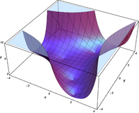
Plots

ℜ[Ai(x+iy)]{displaystyle Re left[mathrm {Ai} (x+iy)right]}	ℑ[Ai(x+iy)]{displaystyle Im left[mathrm {Ai} (x+iy)right]}	|Ai(x+iy)|{displaystyle |mathrm {Ai} (x+iy)|,}	arg[Ai(x+iy)]{displaystyle mathrm {arg} left[mathrm {Ai} (x+iy)right],}

ℜ[Bi(x+iy)]{displaystyle Re left[mathrm {Bi} (x+iy)right]}	ℑ[Bi(x+iy)]{displaystyle Im left[mathrm {Bi} (x+iy)right]}	|Bi(x+iy)|{displaystyle |mathrm {Bi} (x+iy)|,}	arg[Bi(x+iy)]{displaystyle mathrm {arg} left[mathrm {Bi} (x+iy)right],}

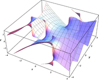Relation to other special functions

For positive arguments, the Airy functions are related to the modified Bessel functions:

Ai(x)=1πx3K13(23x32),Bi(x)=x3(I13(23x32)+I−13(23x32)).{displaystyle {begin{aligned}mathrm {Ai} (x)&{}={frac {1}{pi }}{sqrt {frac {x}{3}}},K_{frac {1}{3}}left({tfrac {2}{3}}x^{frac {3}{2}}right),\mathrm {Bi} (x)&{}={sqrt {frac {x}{3}}}left(I_{frac {1}{3}}left({tfrac {2}{3}}x^{frac {3}{2}}right)+I_{-{frac {1}{3}}}left({tfrac {2}{3}}x^{frac {3}{2}}right)right).end{aligned}}}

Here, I_±1/3 and K_1/3 are solutions of

x2y″+xy′−(x2+19)y=0.{displaystyle x^{2}y''+xy'-left(x^{2}+{tfrac {1}{9}}right)y=0.}

The first derivative of Airy function is

Ai′(x)=−xπ3K23(23x32).{displaystyle mathrm {Ai'} (x)=-{frac {x}{pi {sqrt {3}}}},K_{frac {2}{3}}left({tfrac {2}{3}}x^{frac {3}{2}}right).}

Functions K_1/3 and K_2/3 can be represented in terms of rapidly converged integrals^[4] (see also modified Bessel functions )

For negative arguments, the Airy function are related to the Bessel functions:

Ai(−x)=x9(J13(23x32)+J−13(23x32)),Bi(−x)=x3(J−13(23x32)−J13(23x32)).{displaystyle {begin{aligned}mathrm {Ai} (-x)&{}={sqrt {frac {x}{9}}}left(J_{frac {1}{3}}left({tfrac {2}{3}}x^{frac {3}{2}}right)+J_{-{frac {1}{3}}}left({tfrac {2}{3}}x^{frac {3}{2}}right)right),\mathrm {Bi} (-x)&{}={sqrt {frac {x}{3}}}left(J_{-{frac {1}{3}}}left({tfrac {2}{3}}x^{frac {3}{2}}right)-J_{frac {1}{3}}left({tfrac {2}{3}}x^{frac {3}{2}}right)right).end{aligned}}}

Here, J_±1/3 are solutions of

x2y″+xy′+(x2−19)y=0.{displaystyle x^{2}y''+xy'+left(x^{2}-{tfrac {1}{9}}right)y=0.}

The Scorer's functions Hi(x) and -Gi(x) solve the equation y′′ − xy = 1/π. They can also be expressed in terms of the Airy functions:

Gi(x)=Bi(x)∫x∞Ai(t)dt+Ai(x)∫0xBi(t)dt,Hi(x)=Bi(x)∫−∞xAi(t)dt−Ai(x)∫−∞xBi(t)dt.{displaystyle {begin{aligned}mathrm {Gi} (x)&{}=mathrm {Bi} (x)int _{x}^{infty }mathrm {Ai} (t),dt+mathrm {Ai} (x)int _{0}^{x}mathrm {Bi} (t),dt,\mathrm {Hi} (x)&{}=mathrm {Bi} (x)int _{-infty }^{x}mathrm {Ai} (t),dt-mathrm {Ai} (x)int _{-infty }^{x}mathrm {Bi} (t),dt.end{aligned}}}

Fourier transform

Using the definition of the Airy function Ai(x), it is straightforward to show its Fourier transform is given by

F(Ai)(k):=∫−∞∞Ai(x) e−2πikxdx=ei3(2πk)3.{displaystyle {mathcal {F}}(mathrm {Ai} )(k):=int _{-infty }^{infty }mathrm {Ai} (x) e^{-2pi ikx},dx=e^{{frac {i}{3}}(2pi k)^{3}}.}

Other uses of the term Airy function

Transmittance of a Fabry–Pérot interferometer

"Airy function" in the meaning of the Fabry-Pérot interferometer transmittance.

The transmittance function of a Fabry–Pérot interferometer is also referred to as the Airy Function:^[5]

Te=11+Fsin2⁡(δ2),{displaystyle T_{e}={frac {1}{1+Fsin ^{2}({frac {delta }{2}})}},}

where both surfaces have reflectance R and

F=4R(1−R)2{displaystyle F={frac {4R}{(1-R)^{2}}}}

is the coefficient of finesse.

Diffraction on a circular aperture

"Airy function" in the meaning of the diffraction on circular aperture.

Independently, as a third meaning of the term, the shape of the Airy disk resulting from the wave diffraction on a circular aperture is sometimes also denoted as the Airy function (see e.g. here). This kind of function is closely related to the Bessel function.

History

The Airy function is named after the British astronomer and physicist George Biddell Airy (1801–1892), who encountered it in his early study of optics in physics (Airy 1838). The notation Ai(x) was introduced by Harold Jeffreys. Airy had become the British Astronomer Royal in 1835, and he held that post until his retirement in 1881.

See also

• The proof of Witten's conjecture used a matrix-valued generalization of the Airy function.


• Airy zeta function

Notes

References

• 
  Abramowitz, Milton; Stegun, Irene Ann, eds. (1983) [June 1964]. "Chapter 10". Handbook of Mathematical Functions with Formulas, Graphs, and Mathematical Tables. Applied Mathematics Series. 55 (Ninth reprint with additional corrections of tenth original printing with corrections (December 1972); first ed.). Washington D.C.; New York: United States Department of Commerce, National Bureau of Standards; Dover Publications. p. 446. ISBN 978-0-486-61272-0. LCCN 64-60036. MR 0167642. LCCN 65-12253.
  


• 
  Airy (1838), "On the intensity of light in the neighbourhood of a caustic", Transactions of the Cambridge Philosophical Society, University Press, 6: 379–402, Bibcode:1838TCaPS...6..379A
  


• 
  Frank William John Olver (1974). Asymptotics and Special Functions, Chapter 11. Academic Press, New York.


• 
  Press, WH; Teukolsky, SA; Vetterling, WT; Flannery, BP (2007), "Section 6.6.3. Airy Functions", Numerical Recipes: The Art of Scientific Computing (3rd ed.), New York: Cambridge University Press, ISBN 978-0-521-88068-8
  


• 
  Vallée, Olivier; Soares, Manuel (2004), Airy functions and applications to physics, London: Imperial College Press, ISBN 978-1-86094-478-9, MR 2114198
  

External links

• 
  Hazewinkel, Michiel, ed. (2001) [1994], "Airy functions", Encyclopedia of Mathematics, Springer Science+Business Media B.V. / Kluwer Academic Publishers, ISBN 978-1-55608-010-4
  


• Weisstein, Eric W. "Airy Functions". MathWorld.


• Wolfram function pages for Ai and Bi functions. Includes formulas, function evaluator, and plotting calculator.


• 
  Olver, F. W. J. (2010), "Airy and related functions", in Olver, Frank W. J.; Lozier, Daniel M.; Boisvert, Ronald F.; Clark, Charles W., NIST Handbook of Mathematical Functions, Cambridge University Press, ISBN 978-0521192255, MR 2723248