Rearuh

In probability theory, the expected value of a random variable, intuitively, is the long-run average value of repetitions of the experiment it represents. For example, the expected value in rolling a six-sided die is 3.5, because the average of all the numbers that come up in an extremely large number of rolls is close to 3.5. Less roughly, the law of large numbers states that the arithmetic mean of the values almost surely converges to the expected value as the number of repetitions approaches infinity. The expected value is also known as the expectation, mathematical expectation, EV, average, mean value, mean, or first moment.

More practically, the expected value of a discrete random variable is the probability-weighted average of all possible values. In other words, each possible value the random variable can assume is multiplied by its probability of occurring, and the resulting products are summed to produce the expected value. The same principle applies to an absolutely continuous random variable, except that an integral of the variable with respect to its probability density replaces the sum. The formal definition subsumes both of these and also works for distributions which are neither discrete nor absolutely continuous; the expected value of a random variable is the integral of the random variable with respect to its probability measure.^[1]^[2]

The expected value does not exist for random variables having some distributions with large "tails", such as the Cauchy distribution.^[3] For random variables such as these, the long-tails of the distribution prevent the sum or integral from converging.

The expected value is a key aspect of how one characterizes a probability distribution; it is one type of location parameter. By contrast, the variance is a measure of dispersion of the possible values of the random variable around the expected value. The variance itself is defined in terms of two expectations: it is the expected value of the squared deviation of the variable's value from the variable's expected value.

The expected value plays important roles in a variety of contexts. In regression analysis, one desires a formula in terms of observed data that will give a "good" estimate of the parameter giving the effect of some explanatory variable upon a dependent variable. The formula will give different estimates using different samples of data, so the estimate it gives is itself a random variable. A formula is typically considered good in this context if it is an unbiased estimator— that is if the expected value of the estimate (the average value it would give over an arbitrarily large number of separate samples) can be shown to equal the true value of the desired parameter.

In decision theory, and in particular in choice under uncertainty, an agent is described as making an optimal choice in the context of incomplete information. For risk neutral agents, the choice involves using the expected values of uncertain quantities, while for risk averse agents it involves maximizing the expected value of some objective function such as a von Neumann–Morgenstern utility function. One example of using expected value in reaching optimal decisions is the Gordon–Loeb model of information security investment. According to the model, one can conclude that the amount a firm spends to protect information should generally be only a small fraction of the expected loss (i.e., the expected value of the loss resulting from a cyber or information security breach).^[4]

2 Basic properties
- 2.1 ${displaystyle operatorname {E} [{mathbf {1} }_{A}]=operatorname {P} (A)}$
- 2.2 If $X=Y$ (a.s.) then ${displaystyle operatorname {E} [X]=operatorname {E} [Y]}$
- 2.3 Expected value of a constant
- 2.4 Linearity
- 2.5 $operatorname {E} [X]$ is finite if and only if ${displaystyle operatorname {E} |X|}$ is
- 2.6 If ${displaystyle Xgeq 0}$ (a.s.) then ${displaystyle operatorname {E} [X]geq 0}$
- 2.7 Monotonicity
- 2.8 If ${displaystyle |X|leq Y}$ (a.s.) and ${displaystyle operatorname {E} [Y]}$ is finite then so is $operatorname {E} [X]$
- 2.9 If ${displaystyle operatorname {E} |X^{beta }|<infty }$ and ${displaystyle 0<alpha <beta }$ then ${displaystyle operatorname {E} |X^{alpha }|<infty }$
  - 2.9.1 Counterexample for infinite measure
- 2.10 Extremal property
- 2.11 Non-degeneracy
- 2.12 If ${displaystyle operatorname {E} [X]<+infty }$ then ${displaystyle X<+infty }$ (a.s.)
  - 2.12.1 Corollary: if ${displaystyle operatorname {E} [X]>-infty }$ then ${displaystyle X>-infty }$ (a.s.)
  - 2.12.2 Corollary: if ${displaystyle operatorname {E} |X|<infty }$ then ${displaystyle Xneq pm infty }$ (a.s.)
- 2.13 ${displaystyle |operatorname {E} [X]|leq operatorname {E} |X|}$
- 2.14 Non-multiplicativity
- 2.15 Counterexample: ${displaystyle operatorname {E} [X_{i}]not to operatorname {E} [X]}$ despite ${displaystyle X_{i}to X}$ pointwise
- 2.16 Countable non-additivity
- 2.17 Countable additivity for non-negative random variables

3 ${displaystyle operatorname {E} [XY]=operatorname {E} [X]operatorname {E} [Y]}$ for independent $X$ and $Y$

4 Inequalities
- 4.1 Cauchy–Bunyakovsky–Schwarz inequality
- 4.2 Markov's inequality
- 4.3 Bienaymé-Chebyshev inequality
- 4.4 Jensen's inequality
- 4.5 Lyapunov’s inequality
- 4.6 Hölder’s inequality
- 4.7 Minkowski inequality

5 Taking limits under the $operatorname {E}$ sign
- 5.1 Monotone convergence theorem
- 5.2 Fatou's lemma
- 5.3 Dominated convergence theorem

6 Relationship with characteristic function

7 Uses and applications

8 The law of the unconscious statistician

9 Alternative formula for expected value
- 9.1 Formula for non-negative random variables
  - 9.1.1 Finite and countably infinite case
    - 9.1.1.1 Example
  - 9.1.2 General case
- 9.2 Formula for non-positive random variables
- 9.3 General case

10 History

11 See also

12 Notes

13 Literature

Definition

Finite case

Let $X$ be a random variable with a finite number of finite outcomes $x_{1}$ , $x_{2}$ , ..., $x_{k}$ occurring with probabilities $p_{1}$ , $p_{2}$ , ..., $p_{k}$ , respectively. The expectation of $X$ is defined as

{displaystyle operatorname {E} [X]=sum _{i=1}^{k}x_{i},p_{i}=x_{1}p_{1}+x_{2}p_{2}+cdots +x_{k}p_{k}}

.

Since all probabilities $p_{i}$ add up to 1 ( ${displaystyle p_{1}+p_{2}+ldots +p_{k}=1}$ ), the expected value is the weighted average, with $p_{i}$ ’s being the weights.

If all outcomes $x_{i}$ are equiprobable (that is, ${displaystyle p_{1}=p_{2}=ldots =p_{k}}$ ), then the weighted average turns into the simple average. This is intuitive: the expected value of a random variable is the average of all values it can take; thus the expected value is what one expects to happen on average. If the outcomes $x_{i}$ are not equiprobable, then the simple average must be replaced with the weighted average, which takes into account the fact that some outcomes are more likely than the others. The intuition however remains the same: the expected value of $X$ is what one expects to happen on average.

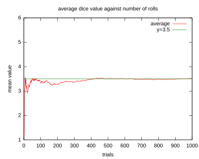
An illustration of the convergence of sequence averages of rolls of a die to the expected value of 3.5 as the number of rolls (trials) grows.

Examples

Let $X$ represent the outcome of a roll of a fair six-sided die. More specifically, $X$ will be the number of pips showing on the top face of the die after the toss. The possible values for $X$ are 1, 2, 3, 4, 5, and 6, all equally likely (each having the probability of 1/6). The expectation of $X$ is

{displaystyle operatorname {E} [X]=1cdot {frac {1}{6}}+2cdot {frac {1}{6}}+3cdot {frac {1}{6}}+4cdot {frac {1}{6}}+5cdot {frac {1}{6}}+6cdot {frac {1}{6}}=3.5.}

If one rolls the die

n

times and computes the average (arithmetic mean) of the results, then as

n

grows, the average will almost surely converge to the expected value, a fact known as the strong law of large numbers. One example sequence of ten rolls of the die is 2, 3, 1, 2, 5, 6, 2, 2, 2, 6, which has the average of 3.1, with the distance of 0.4 from the expected value of 3.5. The convergence is relatively slow: the probability that the average falls within the range

3.5 \pm 0.1

is 21.6% for ten rolls, 46.1% for a hundred rolls and 93.7% for a thousand rolls. See the figure for an illustration of the averages of longer sequences of rolls of the die and how they converge to the expected value of 3.5. More generally, the rate of convergence can be roughly quantified by e.g. Chebyshev's inequality and the Berry–Esseen theorem.

The roulette game consists of a small ball and a wheel with 38 numbered pockets around the edge. As the wheel is spun, the ball bounces around randomly until it settles down in one of the pockets. Suppose random variable $X$ represents the (monetary) outcome of a $1 bet on a single number ("straight up" bet). If the bet wins (which happens with probability 1/38 in American roulette), the payoff is $35; otherwise the player loses the bet. The expected profit from such a bet will be

{displaystyle operatorname {E} [,{text{gain from }}$1{text{ bet}},]=-$1cdot {frac {37}{38}}+$35cdot {frac {1}{38}}=-$0.0526.}

That is, the bet of $1 stands to lose $0.0526, so its expected value is -$0.0526.

Countably infinite case

Let $X$ be a random variable with a countable set of finite outcomes $x_{1}$ , $x_{2}$ , ..., occurring with probabilities $p_{1}$ , $p_{2}$ , ..., respectively,
such that the infinite sum ${displaystyle textstyle sum _{i=1}^{infty }|x_{i}|,p_{i}}$ converges. The expected value of $X$ is defined as the series

{displaystyle operatorname {E} [X]=sum _{i=1}^{infty }x_{i},p_{i}}

.

Remark 1. Observe that ${displaystyle textstyle {Bigl |}operatorname {E} [X]{Bigr |}leq sum _{i=1}^{infty }|x_{i}|,p_{i}<infty }$ .

Remark 2. Due to absolute convergence, the expected value does not depend on the order in which the outcomes are presented. By contrast, a conditionally convergent series can be made to converge or diverge arbitrarily, via the Riemann rearrangement theorem.

Example

Suppose ${displaystyle x_{i}=i}$ and ${displaystyle p_{i}={frac {k}{i2^{i}}},}$ for ${displaystyle i=1,2,3,ldots }$ , where ${displaystyle k={frac {1}{ln 2}}}$ (with $ln$ being the natural logarithm) is the scale factor such that the probabilities sum to 1. Then

{displaystyle operatorname {E} [X]=1left({frac {k}{2}}right)+2left({frac {k}{8}}right)+3left({frac {k}{24}}right)+dots ={frac {k}{2}}+{frac {k}{4}}+{frac {k}{8}}+dots =k.}

Since this series converges absolutely, the expected value of

X

is

k

.

For an example that is not absolutely convergent, suppose random variable $X$ takes values 1, −2, 3, −4, ..., with respective probabilities ${displaystyle {frac {c}{1^{2}}},{frac {c}{2^{2}}},{frac {c}{3^{2}}},{frac {c}{4^{2}}}}$ , ..., where ${displaystyle c={frac {6}{pi ^{2}}}}$ is a normalizing constant that ensures the probabilities sum up to one. Then the infinite sum

sum _{i=1}^{infty }x_{i},p_{i}=c,{bigg (}1-{frac {1}{2}}+{frac {1}{3}}-{frac {1}{4}}+dotsb {bigg )}

converges and its sum is equal to

{displaystyle {frac {6ln 2}{pi ^{2}}}approx 0.421383}

. However it would be incorrect to claim that the expected value of

X

is equal to this number—in fact

operatorname {E} [X]

does not exist (finite or infinite), as this series does not converge absolutely (see Alternating harmonic series).

An example that diverges arises in the context of the St. Petersburg paradox. Let ${displaystyle x_{i}=2^{i}}$ and ${displaystyle p_{i}={frac {1}{2^{i}}}}$ for ${displaystyle i=1,2,3,ldots }$ . The expected value calculation gives

{displaystyle sum _{i=1}^{infty }x_{i},p_{i}=2cdot {frac {1}{2}}+4cdot {frac {1}{4}}+8cdot {frac {1}{8}}+16cdot {frac {1}{16}}+cdots =1+1+1+1+cdots ,.}

Since this does not converge but instead keeps growing, the expected value is infinite.

Absolutely continuous case

If $X$ is a random variable whose cumulative distribution function admits a density $f(x)$ , then the expected value is defined as the following Lebesgue integral:

{displaystyle operatorname {E} [X]=int _{mathbb {R} }xf(x),dx.}

Remark. From computational perspective, the integral in the definition of $operatorname {E} [X]$ may often be treated as an improper Riemann integral ${displaystyle textstyle int _{-infty }^{+infty }xf(x),dx.}$ Specifically, if the function ${displaystyle xf(x)}$ is Riemann-integrable on every finite interval $[a,b]$ , and

{displaystyle min left((-1)cdot {hbox{(R)}}int _{-infty }^{0}xf(x),dx, {hbox{(R)}}int _{0}^{+infty }xf(x),dxright)<infty ,}

then the values (whether finite or infinite) of both integrals agree.

General case

In general, if $X$ is a random variable defined on a probability space ${displaystyle (Omega ,Sigma ,operatorname {P} )}$ , then the expected value of $X$ , denoted by $operatorname {E} [X]$ , ${displaystyle langle Xrangle }$ , or ${bar {X}}$ , is defined as the Lebesgue integral

{displaystyle operatorname {E} [X]=int _{Omega }X(omega ),doperatorname {P} (omega ).}

Remark 1. If ${displaystyle X_{+}(omega )=max(X(omega ),0)}$ and ${displaystyle X_{-}(omega )=-min(X(omega ),0)}$ , then ${displaystyle X=X_{+}-X_{-}.}$ The functions $X_{+}$ and ${displaystyle X_{-}}$ can be shown to be measurable (hence, random variables), and, by definition of Lebesgue integral,

{displaystyle {begin{aligned}operatorname {E} [X]&=int _{Omega }X(omega ),doperatorname {P} (omega )\&=int _{Omega }X_{+}(omega ),doperatorname {P} (omega )-int _{Omega }X_{-}(omega ),doperatorname {P} (omega )\&=operatorname {E} [X_{+}]-operatorname {E} [X_{-}],end{aligned}}}

where ${displaystyle operatorname {E} [X_{+}]}$ and ${displaystyle operatorname {E} [X_{-}]}$ are non-negative and possibly infinite.

The following scenarios are possible:

$operatorname {E} [X]$ is finite, i.e. ${displaystyle max(operatorname {E} [X_{+}],operatorname {E} [X_{-}])<infty ;}$

$operatorname {E} [X]$ is infinite, i.e. ${displaystyle max(operatorname {E} [X_{+}],operatorname {E} [X_{-}])=infty }$ and ${displaystyle min(operatorname {E} [X_{+}],operatorname {E} [X_{-}])<infty ;}$

$operatorname {E} [X]$ is neither finite nor infinite, i.e. ${displaystyle operatorname {E} [X_{+}]=operatorname {E} [X_{-}]=infty .}$

Remark 2. If ${displaystyle F_{X}(x)=operatorname {P} (Xleq x)}$ is the cumulative distribution function of $X$ , then

{displaystyle operatorname {E} [X]=int _{-infty }^{+infty }x,dF_{X}(x),}

where the integral is interpreted in the sense of Lebesgue–Stieltjes.

Remark 3. An example of a distribution for which there is no expected value is Cauchy distribution.

Remark 4. For multidimensional random variables, their expected value is defined per component, i.e.

{displaystyle operatorname {E} [(X_{1},ldots ,X_{n})]=(operatorname {E} [X_{1}],ldots ,operatorname {E} [X_{n}])}

and, for a random matrix $X$ with elements $X_{ij}$ ,

{displaystyle (operatorname {E} [X])_{ij}=operatorname {E} [X_{ij}]}

.

Basic properties

The properties below replicate or follow immediately from those of Lebesgue integral.

${displaystyle operatorname {E} [{mathbf {1} }_{A}]=operatorname {P} (A)}$

If $A$ is an event, then ${displaystyle operatorname {E} [{mathbf {1} }_{A}]=operatorname {P} (A),}$ where ${displaystyle {mathbf {1} }_{A}}$ is the indicator function of the set $A$ .

Proof. By definition of Lebesgue integral of the simple function ${displaystyle {mathbf {1} }_{A}={mathbf {1} }_{A}(omega )}$ ,

{displaystyle operatorname {E} [{mathbf {1} }_{A}]=1cdot operatorname {P} (A)+0cdot operatorname {P} (Omega setminus A)=operatorname {P} (A)}

.

If $X=Y$ (a.s.) then ${displaystyle operatorname {E} [X]=operatorname {E} [Y]}$

The statement follows from the definition of Lebesgue integral if we notice that ${displaystyle X_{+}=Y_{+}}$ (a.s.), ${displaystyle X_{-}=Y_{-}}$ (a.s.), and that changing a simple random variable on a set of probability zero does not alter the expected value.

Expected value of a constant

If $X$ is a random variable, and ${displaystyle X=c}$ (a.s.), where ${displaystyle cin [-infty ,+infty ]}$ , then ${displaystyle operatorname {E} [X]=c}$ . In particular, for an arbitrary random variable $X$ , ${displaystyle operatorname {E} [operatorname {E} [X]]=operatorname {E} [X]}$ .

Proof.

Let $C$ be a constant random variable, i.e. ${displaystyle Cequiv c}$ . It follows from the definition of Lebesgue integral that ${displaystyle operatorname {E} [C]=c}$ . It also follows that ${displaystyle X=C}$ (a.s.). By the previous property,

{displaystyle operatorname {E} [X]=operatorname {E} [C]=c}

.

Linearity

The expected value operator (or expectation operator) $operatorname {E}[cdot ]$ is linear in the sense that

{displaystyle {begin{aligned}operatorname {E} [X+Y]&=operatorname {E} [X]+operatorname {E} [Y],\[6pt]operatorname {E} [aX]&=aoperatorname {E} [X],end{aligned}}}

where $X$ and $Y$ are (arbitrary) random variables, and $a$ is a scalar.

More rigorously, let $X$ and $Y$ be random variables whose expected values are defined (different from $infty -infty$ ).

If ${displaystyle operatorname {E} [X]+operatorname {E} [Y]}$ is also defined (i.e. differs from $infty -infty$ ), then

{displaystyle operatorname {E} [X+Y]=operatorname {E} [X]+operatorname {E} [Y].}

Let ${displaystyle operatorname {E} [X]}$ be finite, and $ain mathbb{R}$ be a finite scalar. Then ${displaystyle operatorname {E} [aX]=aoperatorname {E} [X].}$

Proof.

1. We prove additivity in several steps.

1a. If $X$ and $Y$ are simple and non-negative, taking intersections where necessary, one can re-write $X$ and $Y$ in the form

{displaystyle X=sum _{i=1}^{n}x_{i}cdot {mathbf {1} }_{A_{i}}}

and

{displaystyle Y=sum _{i=1}^{n}y_{i}cdot {mathbf {1} }_{A_{i}}}

,

for some measurable pairwise-disjoint sets ${displaystyle {A_{i}}_{i=1}^{n}}$ partitioning $Omega$ , and ${displaystyle {mathbf {1} }_{A_{i}}={mathbf {1} }_{A_{i}}(omega )}$ being the indicator function of the set $A_{i}$ . By a straightforward check, the additivity follows.

1b. Assuming that $X$ and $Y$ are arbitrary and non-negative, recall that every non-negative measurable function is a pointwise limit of a pointwise non-decreasing sequence of simple non-negative ones. Let ${X_{n}}$ and ${displaystyle {Y_{n}}}$ be such sequences converging to $X$ and $Y,$ respectively. We see that ${displaystyle {X_{n}+Y_{n}}}$ pointwise non-decreases, and ${displaystyle X_{n}+Y_{n}to X+Y}$ pointwise. By monotone convergence theorem and case 1a,

{displaystyle {begin{aligned}operatorname {E} [X+Y]&=operatorname {E} [lim _{n}(X_{n}+Y_{n})]\&=lim _{n}operatorname {E} [X_{n}+Y_{n}]\&=lim _{n}(operatorname {E} [X_{n}]+operatorname {E} [Y_{n}])\&=lim _{n}operatorname {E} [X_{n}]+lim _{n}operatorname {E} [Y_{n}]\&=operatorname {E} [lim _{n}X_{n}]+operatorname {E} [lim _{n}Y_{n}]\&=operatorname {E} [X]+operatorname {E} [Y].end{aligned}}}

(The reader can verify that using the monotone convergence theorem this way does not lead to circular logic).

1c. In the general case, if ${displaystyle Z=X+Y}$ , then ${displaystyle Z_{+}+X_{-}+Y_{-}=Z_{-}+X_{+}+Y_{+},}$
and

{displaystyle operatorname {E} [Z_{+}+X_{-}+Y_{-}]=operatorname {E} [Z_{-}+X_{+}+Y_{+}].}

Splitting up,

{displaystyle operatorname {E} [Z_{+}]+operatorname {E} [X_{-}]+operatorname {E} [Y_{-}]=operatorname {E} [Z_{-}]+operatorname {E} [X_{+}]+operatorname {E} [Y_{+}],}

which is equivalent to,

{displaystyle operatorname {E} [Z_{+}]-operatorname {E} [Z_{-}]=operatorname {E} [X_{+}]+operatorname {E} [Y_{+}]-operatorname {E} [X_{-}]-operatorname {E} [Y_{-}],}

and finally,

{displaystyle operatorname {E} [Z]=operatorname {E} [X]+operatorname {E} [Y].}

2. To prove homogeneity, we first assume that the scalar $a$ above is non-negative. The finiteness of ${displaystyle operatorname {E} [X]}$ implies that $X$ is finite (a.s.). Therefore, ${displaystyle acdot X}$ is also finite (a.s.), which guarantees that ${displaystyle operatorname {E} [aX]}$ is finite. The equality, thus, is a straightforward check based on the definition of Lebesgue integral.

If ${displaystyle a<0}$ , then we first prove that ${displaystyle operatorname {E} [-X]=-operatorname {E} [X]}$ by observing that ${displaystyle (-X)_{+}=X_{-}}$ and vice versa.

$operatorname {E} [X]$ is finite if and only if ${displaystyle operatorname {E} |X|}$ is

The following statements regarding a random variable $X$ are equivalent:

$operatorname {E} [X]$ is finite.

Both ${displaystyle operatorname {E} [X_{+}]}$ and ${displaystyle operatorname {E} [X_{-}]}$ are finite.

${displaystyle operatorname {E} |X|}$ is finite.

Sketch of proof. Indeed, ${displaystyle |X|=X_{+}+X_{-}}$ . By linearity, ${displaystyle operatorname {E} |X|=operatorname {E} [X_{+}]+operatorname {E} [X_{-}]}$ . The above equivalency relies on the definition of Lebesgue integral and measurability of $X$ .

Remark. For the reasons above, the expressions " $X$ is integrable" and "the expected value of $X$ is finite" are used interchangeably when speaking of a random variable throughout this article.

If ${displaystyle Xgeq 0}$ (a.s.) then ${displaystyle operatorname {E} [X]geq 0}$

Proof.

Denote

{displaystyle operatorname {SF} ={s:Omega to mathbb {R} mid s {text{is a simple random variable, and}} 0leq sleq X_{+}}.}

If ${displaystyle sin operatorname {SF} }$ , then ${displaystyle operatorname {E} [s]in [0,+infty )}$ ,
and hence, by definition of Lebesgue integral,

{displaystyle operatorname {E} [X_{+}]=sup _{sin operatorname {SF} }operatorname {E} [s]geq 0}

.

On the other hand, ${displaystyle X_{-}=0}$ (a.s.), so, through a similar argument, ${displaystyle operatorname {E} [X_{-}]=0}$ , and therefore
${displaystyle operatorname {E} [X]=operatorname {E} [X_{+}]-operatorname {E} [X_{-}]=operatorname {E} [X_{+}]geq 0}$ .

Monotonicity

If ${displaystyle Xleq Y}$ (a.s.), and both $operatorname {E} [X]$ and ${displaystyle operatorname {E} [Y]}$ exist, then ${displaystyle operatorname {E} [X]leq operatorname {E} [Y]}$ .

Remark. $operatorname {E} [X]$ and ${displaystyle operatorname {E} [Y]}$ exist in the sense that ${displaystyle min(operatorname {E} [X_{+}],operatorname {E} [X_{-}])<infty }$ and ${displaystyle min(operatorname {E} [Y_{+}],operatorname {E} [Y_{-}])<infty .}$

Proof follows from the linearity and the previous property if we set ${displaystyle Z=Y-X}$ and notice that ${displaystyle Zgeq 0}$ (a.s.).

If ${displaystyle |X|leq Y}$ (a.s.) and ${displaystyle operatorname {E} [Y]}$ is finite then so is $operatorname {E} [X]$

Let $X$ and $Y$ be random variables such that ${displaystyle |X|leq Y}$ (a.s.) and ${displaystyle operatorname {E} [Y]<infty }$ . Then ${displaystyle operatorname {E} [X]neq pm infty }$ .

Proof. Due to non-negativity of $|X|$ , ${displaystyle operatorname {E} |X|}$ exists, finite or infinite. By monotonicity, ${displaystyle operatorname {E} |X|leq operatorname {E} [Y]<infty }$ , so ${displaystyle operatorname {E} |X|}$ is finite which, as we saw earlier, is equivalent to $operatorname {E} [X]$ being finite.

If ${displaystyle operatorname {E} |X^{beta }|<infty }$ and ${displaystyle 0<alpha <beta }$ then ${displaystyle operatorname {E} |X^{alpha }|<infty }$

The proposition below will be used to prove the extremal property of
$operatorname {E} [X]$ later on.

Proposition. If $X$ is a random variable, then so is ${displaystyle X^{alpha }}$ , for every $alpha >0$ . If, in addition, ${displaystyle operatorname {E} |X^{beta }|<infty }$ and
${displaystyle 0<alpha <beta }$ , then ${displaystyle operatorname {E} |X^{alpha }|<infty }$ .

Proof.

To see why the first statement holds, observe that

{displaystyle X^{alpha }}

is a composition of

X

with

{displaystyle xmapsto x^{alpha }}

. As a composition of two measurable functions,

{displaystyle X^{alpha }}

is measurable.

To prove the second statement, define

{displaystyle Y(omega )=max(|X(omega )|^{beta },1)}

.

The reader can verify that $Y$ is a random variable and ${displaystyle |X|^{alpha }leq Y}$ . By non-negativity,

{displaystyle {begin{aligned}operatorname {E} [Y]&=int limits _{{omega mid |X(omega )|^{beta }leq 1}}Y,dP+int limits _{{omega mid |X(omega )|^{beta }>1}}Y,dP\[6pt]&=operatorname {P} {bigl (}|X(omega )|^{beta }leq 1{bigr )}+int limits _{{omega mid |X(omega )|^{beta }>1}}|X|^{beta },dP\[6pt]&leq 1+operatorname {E} |X^{beta }|<infty .end{aligned}}}

By monotonicity,

{displaystyle operatorname {E} |X^{alpha }|leq operatorname {E} [Y]leq 1+operatorname {E} |X^{beta }|<infty }

.

Counterexample for infinite measure

The requirement that ${displaystyle operatorname {P} (Omega )<infty }$ is essential. By way of counterexample, consider the measurable space

{displaystyle ([1,+infty ),{mathcal {B}}_{mathbb {R} _{[1,+infty )}},lambda ),}

where ${displaystyle {mathcal {B}}_{mathbb {R} _{[1,+infty )}}}$ is the Borel $sigma$ -algebra on the interval ${displaystyle [1,+infty ),}$ and $lambda$ is the linear Lebesgue measure. The reader can prove that ${displaystyle textstyle int _{[1,+infty )}{frac {1}{x}},dx=infty ,}$ even though ${displaystyle textstyle int _{[1,+infty )}{frac {1}{x^{2}}},dx=1.}$ (Sketch of proof: ${displaystyle textstyle int _{S}{frac {1}{x}},dx}$ and ${displaystyle textstyle int _{S}{frac {1}{x^{2}}},dx}$ define a measure $mu$ on ${displaystyle textstyle [1,+infty )=cup _{n=1}^{infty }[1,n].}$ Use "continuity from below" w.r. to $mu$ and reduce to Riemann integral on each finite subinterval $[1,n]$ ).

Extremal property

Recall, as we proved early on, that if $X$ is a random variable, then so is $X^{2}$ .

Proposition (extremal property of ${displaystyle operatorname {E} [X])}$ ). Let $X$ be a random variable, and ${displaystyle operatorname {E} [X^{2}]<infty }$ . Then ${displaystyle operatorname {E} [X]}$ and ${displaystyle operatorname {Var} [X]}$ are finite, and ${displaystyle operatorname {E} [X]}$ is the best least squares approximation for $X$ among constants. Specifically,

for every ${displaystyle cin mathbb {R} }$ , ${displaystyle textstyle operatorname {E} [X-c]^{2}geq operatorname {Var} [X];}$

equality holds if and only if ${displaystyle c=operatorname {E} [X].}$

( ${displaystyle operatorname {Var} [X]}$ denotes the variance of $X$ ).

Remark (intuitive interpretation of extremal property). In intuitive terms, the extremal property says that if one is asked to predict the outcome of a trial of a random variable $X$ , then $operatorname {E} [X]$ , in some practically useful sense, is one's best bet if no advance information about the outcome is available. If, on the other hand, one does have some advance knowledge ${mathcal {F}}$ regarding the outcome, then — again, in some practically useful sense — one's bet may be improved upon by using conditional expectations ${displaystyle operatorname {E} [Xmid {mathcal {F}}]}$ (of which $operatorname {E} [X]$ is a special case) rather than $operatorname {E} [X]$ .

Proof of proposition. By the above properties, both $operatorname {E} [X]$ and
${displaystyle operatorname {Var} [X]=operatorname {E} [X^{2}]-operatorname {E} ^{2}[X]}$ are finite, and

{displaystyle {begin{aligned}operatorname {E} [X-c]^{2}&=operatorname {E} [X^{2}-2cX+c^{2}]\[6pt]&=operatorname {E} [X^{2}]-2coperatorname {E} [X]+c^{2}\[6pt]&=(c-operatorname {E} [X])^{2}+operatorname {E} [X^{2}]-operatorname {E} ^{2}[X]\[6pt]&=(c-operatorname {E} [X])^{2}+operatorname {Var} [X],end{aligned}}}

whence the extremal property follows.

Non-degeneracy

If ${displaystyle operatorname {E} |X|=0}$ , then ${displaystyle X=0}$ (a.s.).

Proof.

For every positive constant ${displaystyle rin {mathbb {R} }_{>0}}$ , ${displaystyle operatorname {P} (|X|geq r)=0}$ . Indeed,

{displaystyle rcdot {mathbf {1} }_{|X|geq r}leq |X|cdot {mathbf {1} }_{|X|geq r}leq |X|}

,

where ${displaystyle {mathbf {1} }_{|X|geq r}={mathbf {1} }_{|X|geq r}(omega )}$ is the indicator function of the set ${displaystyle {omega in Omega mid |X(omega )|geq r}}$ . By a property above, the finiteness of ${displaystyle operatorname {E} |X|}$ guarantees that the expected values ${displaystyle operatorname {E} [rcdot {mathbf {1} }_{|X|geq r}]}$ and ${displaystyle operatorname {E} [|X|cdot {mathbf {1} }_{|X|geq r}]}$ are also finite. By monotonicity,

{displaystyle rcdot operatorname {P} (|X|geq r)=operatorname {E} [rcdot {mathbf {1} }_{|X|geq r}]leq operatorname {E} [|X|cdot {mathbf {1} }_{|X|geq r}]leq operatorname {E} |X|=0}

.

For some integer $n>0$ , set ${displaystyle textstyle r={frac {1}{n}}}$ . Define
${displaystyle textstyle S_{n}={omega in Omega mid |X(omega )|geq {frac {1}{n}}}}$ ,
and

{displaystyle textstyle S={omega in Omega mid |X(omega )|>0}}

.

The chain of sets

{displaystyle S_{1}subseteq ldots subseteq S_{n}subseteq S_{n+1}subseteq ldots subseteq S}

monotonically non-decreases, and ${displaystyle S=cup _{n=1}^{infty }S_{n}}$ . By "continuity from below",
${displaystyle textstyle operatorname {P} (S)=lim _{n}operatorname {P} (S_{n})}$ . Applying this formula, obtain

{displaystyle operatorname {P} (Xneq 0)=operatorname {P} (|X|>0)=lim _{n}operatorname {P} left(|X|geq {frac {1}{n}}right)=lim _{n}0=0}

,

as required.

If ${displaystyle operatorname {E} [X]<+infty }$ then ${displaystyle X<+infty }$ (a.s.)

Proof.

Since ${displaystyle operatorname {E} [X]}$ is defined (i.e. ${displaystyle min(operatorname {E} [X_{+}],operatorname {E} [X_{-}])<infty }$ ), and ${displaystyle operatorname {E} [X]=operatorname {E} [X_{+}]-operatorname {E} [X_{-}],}$ we know that ${displaystyle operatorname {E} [X_{+}]}$ is finite, and we want to show that ${displaystyle X_{+}<+infty }$ (a.s.). We will show that ${displaystyle operatorname {P} (Omega _{infty })=0,}$ where

{displaystyle Omega _{infty }={omega in Omega mid X_{+}(omega )=+infty }.}

If ${displaystyle Omega _{infty }=emptyset ,}$ then ${displaystyle operatorname {P} (Omega _{infty })=0,}$ and the proof is complete. Assuming that ${displaystyle Omega _{infty }neq emptyset ,}$ define

{displaystyle operatorname {SF} ={smid s {hbox{ is a simple random variable s.t.}} 0leq sleq X_{+}}.}

Given that ${displaystyle {rm {SF}}neq emptyset }$ , pick ${displaystyle fin {rm {SF}}.}$ For every ${displaystyle textstyle n>sup _{Omega }f,}$ define

{displaystyle f_{n}(omega )={begin{cases}n&{hbox{if}} omega in Omega _{infty }\[3pt]f(omega )&{hbox{if}} omega notin Omega _{infty }.end{cases}}}

Clearly, ${displaystyle f_{n}in {rm {SF}},}$ and

{displaystyle operatorname {E} [f_{n}]=ncdot operatorname {P} (Omega _{infty })+h,}

for some constant ${displaystyle hgeq 0}$ independent from $n.$ (One can easily see that, in fact, ${displaystyle h=operatorname {E} [fcdot {mathbf {1} }_{Omega setminus Omega _{infty }}],}$ but this is of no interest to us here).

Suppose that ${displaystyle operatorname {P} (Omega _{infty })>0.}$ The sequence ${displaystyle {operatorname {E} [f_{n}]}}$ strictly increases, so, by definition of Lebesgue integral,

{displaystyle operatorname {E} [X_{+}]=sup _{sin {rm {SF}}}operatorname {E} [s]geq sup _{n>sup _{Omega }f}operatorname {E} [f_{n}]=+infty cdot operatorname {P} (Omega _{infty })+h=+infty ,}

in contradiction with an earlier conclusion that ${displaystyle operatorname {E} [X_{+}]}$ is finite.

Corollary: if ${displaystyle operatorname {E} [X]>-infty }$ then ${displaystyle X>-infty }$ (a.s.)

Corollary: if ${displaystyle operatorname {E} |X|<infty }$ then ${displaystyle Xneq pm infty }$ (a.s.)

${displaystyle |operatorname {E} [X]|leq operatorname {E} |X|}$

For an arbitrary random variable $X$ , ${displaystyle |operatorname {E} [X]|leq operatorname {E} |X|}$ .

Proof. By definition of Lebesgue integral,

{displaystyle {begin{aligned}|operatorname {E} [X]|&={Bigl |}operatorname {E} [X_{+}]-operatorname {E} [X_{-}]{Bigr |}leq {Bigl |}operatorname {E} [X_{+}]{Bigr |}+{Bigl |}operatorname {E} [X_{-}]{Bigr |}\[5pt]&=operatorname {E} [X_{+}]+operatorname {E} [X_{-}]=operatorname {E} [X_{+}+X_{-}]\[5pt]&=operatorname {E} |X|.end{aligned}}}

Note that this result can also be proved based on Jensen's inequality.

Non-multiplicativity

In general, the expected value operator is not multiplicative, i.e. ${displaystyle operatorname {E} [XY]}$ is not necessarily equal to ${displaystyle operatorname {E} [X]cdot operatorname {E} [Y]}$ . Indeed, let $X$ assume the values of 1 and -1 with probability 0.5 each. Then

{displaystyle operatorname {E^{2}} [X]=left({frac {1}{2}}cdot (-1)+{frac {1}{2}}cdot 1right)^{2}=0}

,

and

{displaystyle operatorname {E} [X^{2}]={frac {1}{2}}cdot (-1)^{2}+{frac {1}{2}}cdot 1^{2}=1}

,

so ${displaystyle operatorname {E} [X^{2}]neq operatorname {E^{2}} [X]}$ .

The amount by which the multiplicativity fails is called the covariance:

operatorname {Cov} (X,Y)=operatorname {E} [XY]-operatorname {E} [X]operatorname {E} [Y].

If, however, the random variables ${displaystyle Xin (Omega _{1},{mathcal {F}}_{1},operatorname {P} _{1})}$ and ${displaystyle Yin (Omega _{2},{mathcal {F}}_{2},operatorname {P} _{2})}$ are independent, then ${displaystyle operatorname {E} [XY]=operatorname {E} [X]operatorname {E} [Y]}$ , and ${displaystyle operatorname {Cov} (X,Y)=0}$ .

Counterexample: ${displaystyle operatorname {E} [X_{i}]not to operatorname {E} [X]}$ despite ${displaystyle X_{i}to X}$ pointwise

Let ${displaystyle left([0,1],{mathcal {B}}_{[0,1]},{mathrm {P} }right)}$ be the probability space, where ${displaystyle {mathcal {B}}_{[0,1]}}$ is the Borel $sigma$ -algebra on $[0,1]$ and ${displaystyle {mathrm {P} }}$ the linear Lebesgue measure. For ${displaystyle igeq 1,}$ define a sequence of random variables

{displaystyle X_{i}=icdot {mathbf {1} }_{left[0,{frac {1}{i}}right]}}

and a random variable

{displaystyle X={begin{cases}+infty &{text{if}} x=0\0&{text{otherwise.}}end{cases}}}

on $[0,1]$ , with ${displaystyle {mathbf {1} }_{S}}$ being the indicator function of the set ${displaystyle Ssubseteq [0,1]}$ .

For every ${displaystyle xin [0,1],}$ as ${displaystyle ito +infty ,}$ ${displaystyle X_{i}(x)to X(x),}$ and

{displaystyle operatorname {E} [X_{i}]=icdot {mathrm {P} }left(left[0,{frac {1}{i}}right]right)=icdot {dfrac {1}{i}}=1,}

so ${displaystyle lim _{ito infty }operatorname {E} [X_{i}]=1.}$ On the other hand, ${displaystyle mathop {mathrm {P} } ({0})=0,}$ and hence ${displaystyle operatorname {E} left[Xright]=0.}$

Countable non-additivity

In general, the expected value operator is not $sigma$ -additive, i.e.

{displaystyle operatorname {E} left[sum _{i=0}^{infty }X_{i}right]neq sum _{i=0}^{infty }operatorname {E} [X_{i}].}

By way of counterexample, let ${displaystyle left([0,1],{mathcal {B}}_{[0,1]},{mathrm {P} }right)}$ be the probability space, where ${displaystyle {mathcal {B}}_{[0,1]}}$ is the Borel $sigma$ -algebra on $[0,1]$ and ${displaystyle {mathrm {P} }}$ the linear Lebesgue measure. Define a sequence of random variables ${displaystyle textstyle X_{i}=(i+1)cdot {mathbf {1} }_{left[0,{frac {1}{i+1}}right]}-icdot {mathbf {1} }_{left[0,{frac {1}{i}}right]}}$ on $[0,1]$ , with ${displaystyle {mathbf {1} }_{S}}$ being the indicator function of the set ${displaystyle Ssubseteq [0,1]}$ . For the pointwise sums, we have

{displaystyle sum _{i=0}^{n}X_{i}=(n+1)cdot {mathbf {1} }_{left[0,{frac {1}{n+1}}right]},}

{displaystyle sum _{i=0}^{infty }X_{i}(x)={begin{cases}+infty &{text{if}} x=0\0&{text{otherwise.}}end{cases}}}

By finite additivity,

{displaystyle sum _{i=0}^{infty }operatorname {E} [X_{i}]=lim _{nto infty }sum _{i=0}^{n}operatorname {E} [X_{i}]=lim _{nto infty }operatorname {E} left[sum _{i=0}^{n}X_{i}right]=1.}

On the other hand, ${displaystyle mathop {mathrm {P} } ({0})=0,}$ and hence

{displaystyle operatorname {E} left[sum _{i=0}^{infty }X_{i}right]=0neq 1=sum _{i=0}^{infty }operatorname {E} [X_{i}].}

Countable additivity for non-negative random variables

Let ${displaystyle {X_{i}}_{i=0}^{infty }}$ be non-negative random variables. It follows from monotone convergence theorem that

{displaystyle operatorname {E} left[sum _{i=0}^{infty }X_{i}right]=sum _{i=0}^{infty }operatorname {E} [X_{i}].}

${displaystyle operatorname {E} [XY]=operatorname {E} [X]operatorname {E} [Y]}$ for independent $X$ and $Y$

Let $X$ and $Y$ be independent random variables with finite expectations $operatorname {E} [X]$ and ${displaystyle operatorname {E} [Y]}$ . Then ${displaystyle operatorname {E} [XY]=operatorname {E} [X]operatorname {E} [Y]}$ .

Proof.

1. The case of non-negative ${displaystyle {mathbb {Q} }}$ -valued random variables.

Given a positive integer $n$ , let the random variables ${displaystyle X:Omega _{1}to {mathbb {R} }}$ and ${displaystyle Y:Omega _{2}to {mathbb {R} }}$ assume their values in the set

{displaystyle left{{frac {m}{n}},{mathrel {Big |}},m=0,1,2,3,ldots right}subset {mathbb {Q} }_{geq 0}.}

Then ${displaystyle textstyle X=sum _{mgeq 0}{frac {m}{n}}cdot {mathbf {1} }_{X_{mn}}}$ , ${displaystyle textstyle Y=sum _{mgeq 0}{frac {m}{n}}cdot {mathbf {1} }_{Y_{mn}}}$ , and

{displaystyle {begin{aligned}XY&=mathop {sum _{m_{1}geq 0}} sum limits _{m_{2}geq 0}{frac {m_{1}}{n}}{mathbf {1} }_{X_{m_{1}n}}cdot {frac {m_{2}}{n}}{mathbf {1} }_{Y_{m_{2}n}}\&={frac {1}{n^{2}}}sum _{igeq 0}icdot sum _{m_{1}cdot m_{2}=i}{mathbf {1} }_{X_{m_{1}n}times Y_{m_{2}n}},end{aligned}}}

or equivalently,

{displaystyle XY(omega )={frac {i}{n^{2}}}Longleftrightarrow omega in bigsqcup _{m_{1}m_{2}=i}(X_{m_{1}n}times Y_{m_{2}n}),}

where ${displaystyle {mathbf {1} }_{S}}$ is the indicator function of the set $S$ ,

{displaystyle X_{mn}=left{omega in Omega _{1},{mathrel {Big |}},X(omega )={frac {m}{n}}right},}

{displaystyle Y_{mn}=left{omega in Omega _{2},{mathrel {Big |}},Y(omega )={frac {m}{n}}right},}

and ${displaystyle bigsqcup }$ denotes disjoint union. By definition of expected value,

{displaystyle {begin{aligned}operatorname {E} [XY]&=int limits _{Omega _{1}times Omega _{2}}XYdoperatorname {P} \&={frac {1}{n^{2}}}sum _{igeq 0}icdot sum _{m_{1}cdot m_{2}=i}operatorname {P} (Xin X_{m_{1}n},Yin Y_{m_{2}n})end{aligned}}}

Due to independence,

{displaystyle operatorname {P} (Xin X_{m_{1}n},Yin Y_{m_{2}n})=operatorname {P} (Xin X_{m_{1}n})cdot operatorname {P} (Yin Y_{m_{2}n}),}

whence

{displaystyle {begin{aligned}operatorname {E} [XY]&={frac {1}{n^{2}}}sum _{igeq 0}icdot sum _{m_{1}cdot m_{2}=i}operatorname {P} (Xin X_{m_{1}n})operatorname {P} (Yin Y_{m_{2}n})\[6pt]&=mathop {sum _{m_{1}geq 0}} sum limits _{m_{2}geq 0}{frac {m_{1}}{n}}operatorname {P} (Xin X_{m_{1}n})cdot {frac {m_{2}}{n}}operatorname {P} (Yin Y_{m_{2}n})\[6pt]&=left(sum _{m_{1}geq 0}{frac {m_{1}}{n}}operatorname {P} (Xin X_{m_{1}n})right)cdot left(sum _{m_{2}geq 0}{frac {m_{2}}{n}}operatorname {P} (Yin Y_{m_{2}n})right)\[6pt]&=operatorname {E} [X]operatorname {E} [Y].end{aligned}}}

2. The case of non-negative random variables.

Let $X$ and $Y$ be (arbitrary) non-negative random variable. Define

{displaystyle X_{n}(omega )={begin{cases}{frac {m}{n}}&{text{if}} {frac {m}{n}}leq X(omega )<{frac {m+1}{n}},\[6pt]0&{text{if}} X(omega )=+infty ,end{cases}}}

for an arbitrary ${displaystyle omega in Omega _{1}}$ . Note that ${displaystyle X_{n}:Omega _{1}to {mathbb {R} }}$ is a random variable and

{displaystyle {text{Range}}(X_{n})subseteq left{{frac {m}{n}},{mathrel {Big |}},m=0,1,2,3,ldots right}subset mathbb {Q} _{geq 0}.}

As we saw previously, the finiteness of $operatorname {E} [X]$ implies that $X$ is finite almost sure, and consequently, ${displaystyle textstyle |X_{n}-X|leq {frac {1}{n}}}$ (a.s.) on $Omega _{1}$ . This, in turn, implies that ${displaystyle textstyle operatorname {E} |X_{n}-X|leq {frac {1}{n}}}$ .

Let the random variable $Y_{n}$ be defined the same way but with respect to $Y$ . We have

{displaystyle {begin{aligned}&{Bigl |}operatorname {E} [XY]-operatorname {E} [X]operatorname {E} [Y]{Bigr |}=\&={Bigl |}operatorname {E} [XY]-operatorname {E} [X_{n}Y]+operatorname {E} [X_{n}Y]-operatorname {E} [X]operatorname {E} [Y]{Bigr |}\&={Bigl |}operatorname {E} [(X-X_{n})Y]+operatorname {E} [X_{n}Y]-operatorname {E} [X]operatorname {E} [Y]{Bigr |}\&leq {frac {1}{n}}operatorname {E} |Y|+{Bigl |}operatorname {E} [X_{n}Y]-operatorname {E} [X]operatorname {E} [Y]{Bigr |}\&={frac {1}{n}}operatorname {E} |Y|+{Bigl |}operatorname {E} [X_{n}Y]-operatorname {E} [X_{n}Y_{n}]+operatorname {E} [X_{n}Y_{n}]-operatorname {E} [X]operatorname {E} [Y]{Bigr |}\&leq {frac {1}{n}}operatorname {E} |Y|+{frac {1}{n}}operatorname {E} |X_{n}|+{Bigl |}operatorname {E} [X_{n}Y_{n}]-operatorname {E} [X]operatorname {E} [Y]{Bigr |}\&={frac {1}{n}}operatorname {E} |Y|+{frac {1}{n}}operatorname {E} |X_{n}-X+X|+{Bigl |}operatorname {E} [X_{n}Y_{n}]-operatorname {E} [X]operatorname {E} [Y]{Bigr |}\&leq {frac {1}{n}}operatorname {E} |Y|+{frac {operatorname {E} |X_{n}-X|+operatorname {E} |X|}{n}}+{Bigl |}operatorname {E} [X_{n}Y_{n}]-operatorname {E} [X]operatorname {E} [Y]{Bigr |}\&leq {frac {1}{n}}operatorname {E} |Y|+{frac {1}{n^{2}}}+{frac {operatorname {E} |X|}{n}}+{Bigl |}operatorname {E} [X_{n}Y_{n}]-operatorname {E} [X]operatorname {E} [Y]{Bigr |}.end{aligned}}}

$X_{n}$ and $Y_{n}$ were shown to satisfy ${displaystyle operatorname {E} [X_{n}Y_{n}]=operatorname {E} [X_{n}]operatorname {E} [Y_{n}]}$ . Therefore,

{displaystyle {begin{aligned}&{Bigl |}operatorname {E} [X_{n}Y_{n}]-operatorname {E} [X]operatorname {E} [Y]{Bigr |}=\&={Bigl |}operatorname {E} [X_{n}]operatorname {E} [Y_{n}]-operatorname {E} [X]operatorname {E} [Y]{Bigr |}=\&={Bigl |}operatorname {E} [X_{n}]operatorname {E} [Y_{n}]-operatorname {E} [X]operatorname {E} [Y_{n}]+operatorname {E} [X]operatorname {E} [Y_{n}]-operatorname {E} [X]operatorname {E} [Y]{Bigr |}\&leq {Bigl |}operatorname {E} [X_{n}]operatorname {E} [Y_{n}]-operatorname {E} [X]operatorname {E} [Y_{n}]{Bigr |}+{Bigl |}operatorname {E} [X]operatorname {E} [Y_{n}]-operatorname {E} [X]operatorname {E} [Y]{Bigr |}\&leq operatorname {E} |X_{n}-X|cdot operatorname {E} |Y_{n}|+operatorname {E} |X|cdot operatorname {E} |Y_{n}-Y|\&leq {frac {operatorname {E} |Y_{n}|+operatorname {E} |X|}{n}}={frac {operatorname {E} |Y_{n}-Y+Y|+operatorname {E} |X|}{n}}\&leq {frac {operatorname {E} |Y_{n}-Y|+operatorname {E} |Y|+operatorname {E} |X|}{n}}\&leq {frac {1}{n^{2}}}+{frac {operatorname {E} |Y|+operatorname {E} |X|}{n}}.end{aligned}}}

It follows that, being independent from $n$ , the constant value ${displaystyle {Bigl |}operatorname {E} [XY]-operatorname {E} [X]operatorname {E} [Y]{Bigr |}}$ can only be equal to 0.

3. The general case.

Let $X$ and $Y$ be arbitrary random variables. We have

{displaystyle {begin{aligned}operatorname {E} [XY]&=operatorname {E} [(X_{+}-X_{-})(Y_{+}-Y_{-})]\&=operatorname {E} [X_{+}Y_{+}]-operatorname {E} [X_{+}Y_{-}]-operatorname {E} [X_{-}Y_{+}]+operatorname {E} [X_{-}Y_{-}]\&=operatorname {E} [X_{+}]operatorname {E} [Y_{+}]-operatorname {E} [X_{+}]operatorname {E} [Y_{-}]-operatorname {E} [X_{-}]operatorname {E} [Y_{+}]+operatorname {E} [X_{-}]operatorname {E} [Y_{-}]\&=(operatorname {E} [X_{+}]-operatorname {E} [X_{-}])(operatorname {E} [Y_{+}]-operatorname {E} [Y_{-}])\&=operatorname {E} [X_{+}-X_{-}]operatorname {E} [Y_{+}-Y_{-}]\&=operatorname {E} [X]operatorname {E} [Y].end{aligned}}}

Inequalities

Cauchy–Bunyakovsky–Schwarz inequality

The Cauchy–Bunyakovsky–Schwarz inequality states that

{displaystyle (operatorname {E} [XY])^{2}leq operatorname {E} [X^{2}]cdot operatorname {E} [Y^{2}].}

Markov's inequality

For a nonnegative random variable $X$ and $a>0$ , the Markov's inequality states that

{displaystyle operatorname {P} (Xgeq a)leq {frac {operatorname {E} [X]}{a}}.}

Bienaymé-Chebyshev inequality

Let $X$ be an arbitrary random variable with finite expected value $operatorname {E} [X]$ and finite variance ${displaystyle operatorname {Var} [X]neq 0}$ . The Bienaymé-Chebyshev inequality states that, for any real number $k>0$ ,

{displaystyle operatorname {P} {Bigl (}{Bigl |}X-operatorname {E} [X]{Bigr |}geq k{sqrt {operatorname {Var} [X]}}{Bigr )}leq {frac {1}{k^{2}}}.}

Jensen's inequality

Let ${displaystyle f:{mathbb {R} }to {mathbb {R} }}$ be a Borel convex function and $X$ a random variable such that ${displaystyle operatorname {E} |X|<infty }$ . Jensen's inequality states that

{displaystyle f(operatorname {E} (X))leq operatorname {E} (f(X)).}

Remark 1. The expected value ${displaystyle operatorname {E} (f(X))}$ is well-defined even if $X$ is allowed to assume infinite values. Indeed, ${displaystyle operatorname {E} |X|<infty }$ implies that ${displaystyle Xneq pm infty }$ (a.s.), so the random variable ${displaystyle f(X(omega ))}$ is defined almost sure, and therefore there is enough information to compute ${displaystyle operatorname {E} (f(X)).}$

Remark 2. Jensen's inequality implies that ${displaystyle |operatorname {E} [X]|leq operatorname {E} |X|}$ since the absolute value function is convex.

Lyapunov’s inequality

Let ${displaystyle 0<s<t}$ . Lyapunov's inequality states that

{displaystyle {Bigl (}operatorname {E} |X|^{s}{Bigr )}^{1/s}leq left(operatorname {E} |X|^{t}right)^{1/t}.}

Proof. Applying Jensen's inequality to ${displaystyle |X|^{s}}$ and ${displaystyle g(x)=|x|^{t/s}}$ , obtain
${displaystyle {Bigl |}operatorname {E} |X^{s}|{Bigr |}^{t/s}leq operatorname {E} |X^{s}|^{t/s}=operatorname {E} |X|^{t}}$ . Taking the $t$ th
root of each side completes the proof.

Corollary.

{displaystyle operatorname {E} |X|leq {Bigl (}operatorname {E} |X|^{2}{Bigr )}^{1/2}leq ldots leq {Bigl (}operatorname {E} |X|^{n}{Bigr )}^{1/n}leq ldots }

Hölder’s inequality

Let $p$ and $q$ satisfy ${displaystyle 1leq pleq infty }$ , ${displaystyle 1leq qleq infty }$ , and $1/p+1/q=1$ . The Hölder's inequality states that

{displaystyle operatorname {E} |XY|leq (operatorname {E} |X|^{p})^{1/p}(operatorname {E} |Y|^{q})^{1/q}.}

Minkowski inequality

Let $p$ be an integer satisfying ${displaystyle 1leq pleq infty }$ . Let, in addition, ${displaystyle operatorname {E} |X|^{p}<infty }$ and ${displaystyle operatorname {E} |Y|^{p}<infty }$ . Then, according to the Minkowski inequality, ${displaystyle operatorname {E} |X+Y|^{p}<infty }$ and

{displaystyle {Bigl (}operatorname {E} |X+Y|^{p}{Bigr )}^{1/p}leq {Bigl (}operatorname {E} |X|^{p}{Bigr )}^{1/p}+{Bigl (}operatorname {E} |Y|^{p}{Bigr )}^{1/p}.}

Taking limits under the $operatorname {E}$ sign

Monotone convergence theorem

Let the sequence of random variables ${X_{n}}$ and the random variables $X$ and $Y$ be defined on the same probability space ${displaystyle (Omega ,Sigma ,operatorname {P} ).}$ Suppose that

all the expected values ${displaystyle operatorname {E} [X_{n}],}$ ${displaystyle operatorname {E} [X],}$ and ${displaystyle operatorname {E} [Y]}$ are defined (differ from $infty -infty$ );

${displaystyle operatorname {E} [Y]>-infty ;}$

for every ${displaystyle n,}$

{displaystyle -infty leq Yleq X_{n}leq X_{n+1}leq +infty quad {hbox{(a.s.)}};}

$X$ is the pointwise limit of ${displaystyle {X_{n}}}$ (a.s.), i.e. ${displaystyle X(omega )=lim nolimits _{n}X_{n}(omega )}$ (a.s.).

The monotone convergence theorem states that

${displaystyle lim _{n}operatorname {E} [X_{n}]=operatorname {E} [X].}$

Proof.

Observe that, by monotonicity, the sequence ${displaystyle {operatorname {E} [X_{n}]}}$ monotonically non-decreases, and ${displaystyle operatorname {E} [Y]leq operatorname {E} [X_{n}]leq operatorname {E} [X].}$

If ${displaystyle operatorname {E} [Y]=+infty ,}$ then ${displaystyle operatorname {E} [Y]=operatorname {E} [X_{n}]=operatorname {E} [X],}$ and we are done.

If ${displaystyle operatorname {E} [Y]<+infty ,}$ then, following the assumption that ${displaystyle operatorname {E} [Y]>-infty ,}$ we conclude that ${displaystyle operatorname {E} [Y]}$ is finite which, in turn, implies, as we saw previously, that $Y$ is finite (a.s.).

Denote ${displaystyle Z_{n}=X_{n}-Y}$ and ${displaystyle Z=X-Y}$ . The finiteness of $Y$ (a.s.) implies that the differences ${displaystyle Z_{n}=X_{n}-Y}$ and ${displaystyle Z=X-Y}$ are defined (do not have the form $infty -infty$ ) everywhere outside of a null set. On that null set, $Z_{n}$ and $Z$ may be defined arbitrarily (e.g. as zero or in any other way, as long as measurability is preserved) without affecting this proof. As a difference of two random variables, $Z_{n}$ and $Z$ are also random variables.

It follows from the definition that ${displaystyle Z_{n}geq 0}$ (a.s.), ${displaystyle Zgeq 0}$ (a.s.), the sequence ${displaystyle {Z_{n}}}$ pointwise non-decreases (a.s.), and ${displaystyle Z_{n}to Z}$ pointwise (a.s.).

By (the general version of) monotone convergence theorem,

{displaystyle {begin{aligned}(lim _{n}operatorname {E} [X_{n}])-operatorname {E} [Y]&=lim _{n}(operatorname {E} [X_{n}]-operatorname {E} [Y])\&=lim _{n}operatorname {E} [X_{n}-Y]\&=lim _{n}operatorname {E} [Z_{n}]\&=operatorname {E} [Z]\&=operatorname {E} [X-Y]\&=operatorname {E} [X]-operatorname {E} [Y],end{aligned}}}

whence the assertion follows.

Fatou's lemma

Let the sequence of random variables ${X_{n}}$ and the random variable $Y$ be defined on the same probability space ${displaystyle (Omega ,Sigma ,operatorname {P} ).}$ Suppose that

all the expected values ${displaystyle operatorname {E} [X_{n}],}$ ${displaystyle textstyle operatorname {E} [liminf _{n}X_{n}],}$ and ${displaystyle operatorname {E} [Y]}$ are defined (differ from $infty -infty$ );

${displaystyle operatorname {E} [Y]>-infty ;}$

${displaystyle -infty leq Yleq X_{n}leq +infty }$ (a.s.), for every $n.$

Fatou's lemma states that

{displaystyle operatorname {E} [liminf _{n}X_{n}]leq liminf _{n}operatorname {E} [X_{n}].}

(Note that ${displaystyle textstyle liminf _{n}X_{n}}$ is a random variable, for every ${displaystyle n,}$ by the properties of limit inferior).

Proof.

If ${displaystyle operatorname {E} [Y]=+infty ,}$ then, by monotonicity, ${displaystyle operatorname {E} [Y]=operatorname {E} [X_{n}]=+infty ,}$ so ${displaystyle textstyle liminf _{n}operatorname {E} [X_{n}]=+infty ,}$ and the assertion follows.

If ${displaystyle operatorname {E} [Y]<+infty }$ , then, following the assumption that ${displaystyle operatorname {E} [Y]>-infty ,}$ we conclude that ${displaystyle operatorname {E} [Y]}$ is finite which, in turn, implies, as we saw previously, that $Y$ is finite (a.s.).

Denote ${displaystyle Z_{n}=X_{n}-Y}$ . Then ${displaystyle Z_{n}geq 0}$ (a.s.). The finiteness of $Y$ (a.s.) implies that $Z_{n}$ is defined (does not have the form $infty -infty$ ) everywhere outside of a null set. On that null set $Z_{n}$ may be defined arbitrarily (e.g. as zero or in any other way, as long as measurability is preserved) without affecting this proof. As a difference of two random variables, $Z_{n}$ is a random variable.

By (the general version of) Fatou's lemma,

{displaystyle {begin{aligned}operatorname {E} [liminf _{n}X_{n}]-operatorname {E} [Y]&=operatorname {E} [liminf _{n}(X_{n}-Y)]\&=operatorname {E} [liminf _{n}Z_{n}]\&leq liminf _{n}operatorname {E} [Z_{n}]\&=liminf _{n}operatorname {E} [X_{n}-Y]\&=liminf _{n}(operatorname {E} [X_{n}]-operatorname {E} [Y])\&=(liminf _{n}operatorname {E} [X_{n}])-operatorname {E} [Y],end{aligned}}}

whence the assertion follows.

Corollary. Let

${displaystyle X_{n}to X}$ pointwise (a.s.);

${displaystyle operatorname {E} [X_{n}]leq C,}$ for some constant $C$ (independent from $n$ );

${displaystyle operatorname {E} [Y]>-infty ;}$

${displaystyle -infty leq Yleq X_{n}leq +infty }$ (a.s.), for every $n.$

Then ${displaystyle operatorname {E} [X]leq C.}$

Proof is by observing that ${displaystyle textstyle X=liminf _{n}X_{n}}$ (a.s.) and applying Fatou's lemma.

Dominated convergence theorem

Let ${displaystyle {X_{n}}_{n}}$ be a sequence of random variables. If ${displaystyle X_{n}to X}$ pointwise (a.s.), ${displaystyle |X_{n}|leq Yleq +infty }$ (a.s.), and ${displaystyle operatorname {E} [Y]<infty }$ . Then, according to the dominated convergence theorem,

the function $X$ is measurable (hence a random variable);

${displaystyle operatorname {E} |X|<infty }$ ;

all the expected values ${displaystyle operatorname {E} [X_{n}]}$ and ${displaystyle operatorname {E} [X]}$ are defined (do not have the form ${displaystyle infty -infty }$ );

${displaystyle lim _{n}operatorname {E} [X_{n}]=operatorname {E} [X]}$ (both sides may be infinite);

${displaystyle lim _{n}operatorname {E} |X_{n}-X|=0}$ .

Relationship with characteristic function

The probability density function $f_X$ of a scalar random variable $X$ is related to its characteristic function ${displaystyle varphi _{X}}$ by the inversion formula:

{displaystyle f_{X}(x)={frac {1}{2pi }}int _{mathbb {R} }e^{-itx}varphi _{X}(t),dt.}

For the expected value of $g(X)$ (where ${displaystyle g:{mathbb {R} }to {mathbb {R} }}$ is a Borel function), we can use this inversion formula to obtain

{displaystyle operatorname {E} [g(X)]={frac {1}{2pi }}int _{mathbb {R} }g(x)left[{int _{mathbb {R} }e^{-itx}varphi _{X}(t),dt}right]dx.}

If ${displaystyle operatorname {E} [g(X)]}$ is finite, changing the order of integration, we get, in accordance with Fubini-Tonelli theorem,

{displaystyle operatorname {E} [g(X)]={frac {1}{2pi }}int _{mathbb {R} }G(t)varphi _{X}(t),dt,}

where

{displaystyle G(t)=int _{mathbb {R} }g(x)e^{-itx},dx}

is the Fourier transform of $g(x).$ The expression for ${displaystyle operatorname {E} [g(X)]}$ also follows directly from Plancherel theorem.

Uses and applications

It is possible to construct an expected value equal to the probability of an event by taking the expectation of an indicator function that is one if the event has occurred and zero otherwise. This relationship can be used to translate properties of expected values into properties of probabilities, e.g. using the law of large numbers to justify estimating probabilities by frequencies.

The expected values of the powers of X are called the moments of X; the moments about the mean of X are expected values of powers of X − E[X]. The moments of some random variables can be used to specify their distributions, via their moment generating functions.

To empirically estimate the expected value of a random variable, one repeatedly measures observations of the variable and computes the arithmetic mean of the results. If the expected value exists, this procedure estimates the true expected value in an unbiased manner and has the property of minimizing the sum of the squares of the residuals (the sum of the squared differences between the observations and the estimate). The law of large numbers demonstrates (under fairly mild conditions) that, as the size of the sample gets larger, the variance of this estimate gets smaller.

This property is often exploited in a wide variety of applications, including general problems of statistical estimation and machine learning, to estimate (probabilistic) quantities of interest via Monte Carlo methods, since most quantities of interest can be written in terms of expectation, e.g. ${displaystyle operatorname {P} ({Xin {mathcal {A}}})=operatorname {E} [{mathbf {1} }_{mathcal {A}}]}$ , where ${displaystyle {mathbf {1} }_{mathcal {A}}}$ is the indicator function of the set ${mathcal {A}}$ .

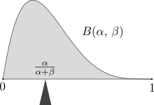
The mass of probability distribution is balanced at the expected value, here a Beta(α,β) distribution with expected value α/(α+β).

In classical mechanics, the center of mass is an analogous concept to expectation. For example, suppose X is a discrete random variable with values x_i and corresponding probabilities p_i. Now consider a weightless rod on which are placed weights, at locations x_i along the rod and having masses p_i (whose sum is one). The point at which the rod balances is E[X].

Expected values can also be used to compute the variance, by means of the computational formula for the variance

operatorname {Var} (X)=operatorname {E} [X^{2}]-(operatorname {E} [X])^{2}.

A very important application of the expectation value is in the field of quantum mechanics. The expectation value of a quantum mechanical operator ${hat {A}}$ operating on a quantum state vector $|psi rangle$ is written as $langle {hat {A}}rangle =langle psi |A|psi rangle$ . The uncertainty in ${hat {A}}$ can be calculated using the formula $(Delta A)^{2}=langle {hat {A}}^{2}rangle -langle {hat {A}}rangle ^{2}$ .

The law of the unconscious statistician

The expected value of a measurable function of $X$ , $g(X)$ , given that $X$ has a probability density function $f(x)$ , is given by the inner product of $f$ and $g$ :

{displaystyle operatorname {E} [g(X)]=int _{mathbb {R} }g(x)f(x),dx.}

This formula also holds in multidimensional case, when $g$ is a function of several random variables, and $f$ is their joint density.^[5]^[6]

Alternative formula for expected value

Formula for non-negative random variables

Finite and countably infinite case

For a non-negative integer-valued random variable ${displaystyle X:Omega to {0,1,2,3,ldots }cup {+infty },}$

{displaystyle operatorname {E} [X]=sum _{i=1}^{infty }operatorname {P} (Xgeq i).}

Proof.

If ${displaystyle operatorname {P} (X=+infty )>0,}$ then ${displaystyle operatorname {E} [X]=+infty .}$ On the other hand,

{displaystyle operatorname {P} (Xgeq i)geq operatorname {P} (X=+infty )>0,}

so the series on the right diverges to ${displaystyle +infty ,}$ and the equality holds.

If ${displaystyle operatorname {P} (X=+infty )=0,}$ then

{displaystyle sum _{i=1}^{infty }operatorname {P} (Xgeq i)=sum _{i=1}^{infty }sum _{j=i}^{infty }operatorname {P} (X=j).}

Let

{displaystyle M={begin{bmatrix}operatorname {P} (X=1)&operatorname {P} (X=2)&operatorname {P} (X=3)&ldots &operatorname {P} (X=n)&ldots \&operatorname {P} (X=2)&operatorname {P} (X=3)&ldots &operatorname {P} (X=n)&ldots \&&operatorname {P} (X=3)&ldots &operatorname {P} (X=n)&ldots \cdots &cdots &cdots &cdots &cdots &cdots \&&&&operatorname {P} (X=n)&cdots \cdots &cdots &cdots &cdots &cdots &cdots end{bmatrix}}}

be an infinite upper triangular matrix. The double series ${displaystyle textstyle sum _{i=1}^{infty }sum _{j=i}^{infty }operatorname {P} (X=j)}$ is the sum of $M$ 's elements if summation is done row by row.
Since every summand is non-negative, the series either converges absolutely or diverges to ${displaystyle +infty .}$ In both cases, changing summation order does not affect the sum. Changing summation order, from row-by-row to column-by-column, gives us

{displaystyle {begin{aligned}sum _{i=1}^{infty }sum _{j=i}^{infty }operatorname {P} (X=j)&=sum _{j=1}^{infty }sum _{i=1}^{j}operatorname {P} (X=j)\&=sum _{j=1}^{infty }joperatorname {P} (X=j)\&=operatorname {E} [X].end{aligned}}}

Example

In a coin tossing experiment, let the probability of heads be $p$ . Including the final attempt, how many tosses can we expect until the first head?

Solution. If $N$ is the random variable indicating the numbers of coin tosses before and including the first head, then, for $igeq 1$ ,

{displaystyle {begin{aligned}operatorname {P} (Ngeq i)&=1-operatorname {P} (Nleq i-1)\[1pt]&=1-sum limits _{j=0}^{i-1}operatorname {P} (N=j)\[1pt]&=1-sum limits _{j=1}^{i-1}(1-p)^{j-1}p\[1pt]&=1-{frac {1-(1-p)^{i-1}}{p}}cdot p\[1pt]&=(1-p)^{i-1},end{aligned}}}

where we took into account the geometric series summation formula. We now compute

{displaystyle {begin{aligned}operatorname {E} [N]&=sum limits _{i=1}^{infty }operatorname {P} (Ngeq i)\&=sum limits _{i=1}^{infty }(1-p)^{i-1}\&={frac {1}{p}}.end{aligned}}}

General case

If ${displaystyle X:Omega to [0,+infty ]}$ is a non-negative random variable, then

{displaystyle operatorname {E} [X]=int limits _{[0,+infty )}operatorname {P} (Xgeq x),dx=int limits _{[0,+infty )}operatorname {P} (X>x),dx,}

and

{displaystyle operatorname {E} [X]={hbox{(R)}}int limits _{0}^{infty }operatorname {P} (Xgeq x),dx={hbox{(R)}}int limits _{0}^{infty }operatorname {P} (X>x),dx,}

where ${displaystyle {hbox{(R)}}textstyle int _{0}^{infty }}$ denotes improper Riemann integral.

Proof.

1. For every $omega in Omega$ ,

{displaystyle X(omega )=int limits _{(0,X(omega ))}dx=int limits _{[0,+infty )}{mathbf {1} }_{(0,X(omega ))}(x),dx=int limits _{[0,+infty )}{mathbf {1} }_{(0,X(omega )]}(x),dx,}

where ${displaystyle {mathbf {1} }_{(0,X(omega ))}}$ and ${displaystyle {mathbf {1} }_{(0,X(omega )]}}$ are the indicator functions of ${displaystyle (0,X(omega ))}$ and ${displaystyle (0,X(omega )]}$ , respectively. Substituting this into the definition of $operatorname {E} [X]$ , obtain

{displaystyle {begin{aligned}operatorname {E} [X]&=int limits _{Omega }Xdoperatorname {P} \&=int limits _{Omega }int limits _{[0,+infty )}{mathbf {1} }_{(0,X(omega )]}(x),dx,doperatorname {P} (omega ).end{aligned}}}

Since ${displaystyle X(omega )geq 0}$ and ${displaystyle {mathbf {1} }_{(0,X(omega )]}(x)geq 0,}$ this integral (finite or infinite) meets the requirements of Tonelli's theorem. Changing the order of integration gives us

{displaystyle {begin{aligned}&int limits _{[0,+infty )}int limits _{Omega }{mathbf {1} }_{(0,X(omega )]}(x),doperatorname {P} (omega ),dx\&=int limits _{[0,+infty )}operatorname {P} (Xgeq x),dx.end{aligned}}}

2a. The function ${displaystyle y(x)=operatorname {P} (Xgeq x)}$ is Riemann-integrable on each finite interval ${displaystyle [a,b].}$ Indeed, since $y(x)$ is non-increasing, the set $D$ of its discontinuities is countable. Due to countable additivity,
$D$ is a null set with respect to the linear Lebesgue measure. Furthermore, ${displaystyle 0leq y(x)leq 1,}$ for all ${displaystyle xin [-infty ,+infty ].}$ Using the Lebesgue criterion, Riemann integrability of $y(x)$ follows. We also conclude that

{displaystyle int limits _{[a,b]}operatorname {P} (Xgeq x),dx={hbox{(R)}}int _{a}^{b}operatorname {P} (Xgeq x),dx.}

2b. By "continuity from below",

{displaystyle {begin{aligned}int limits _{[0,+infty )}operatorname {P} (Xgeq x),dx&=lim _{tto +infty }int limits _{[0,t]}operatorname {P} (Xgeq x),dx\&=lim _{tto +infty }{hbox{(R)}}int limits _{0}^{t}operatorname {P} (Xgeq x),dx\&={hbox{(R)}}int limits _{0}^{infty }operatorname {P} (Xgeq x),dx.end{aligned}}}

The case of ${displaystyle operatorname {P} (X>x)}$ is similar.

Formula for non-positive random variables

If ${displaystyle X:Omega to [-infty ,0]}$ is a non-positive random variable, then

{displaystyle operatorname {E} [X]=-int limits _{(-infty ,0]}operatorname {P} (Xleq x),dx=-int limits _{(-infty ,0]}operatorname {P} (X<x),dx,}

and

{displaystyle operatorname {E} [X]=-{hbox{(R)}}int limits _{-infty }^{0}operatorname {P} (Xleq x),dx=-{hbox{(R)}}int limits _{-infty }^{0}operatorname {P} (X<x),dx,}

where ${displaystyle {hbox{(R)}}textstyle int _{-infty }^{0}}$ denotes improper Riemann integral.

This formula follows from that for the non-negative case applied to ${displaystyle -X.}$

If, in addition, $X$ is integer-valued, i.e. ${displaystyle X:Omega to {ldots ,-3,-2,-1,0}cup {-infty }}$ , then

{displaystyle operatorname {E} [X]=-sum _{i=-1}^{-infty }operatorname {P} (Xleq i).}

General case

If $X$ can be both positive and negative, then ${displaystyle operatorname {E} [X]=operatorname {E} [X_{+}]-operatorname {E} [X_{-}]}$ ,
and the above results may be applied to $X_{+}$ and ${displaystyle X_{-}}$ separately.

History

The idea of the expected value originated in the middle of the 17th century from the study of the so-called problem of points, which seeks to divide the stakes in a fair way between two players who have to end their game before it's properly finished. This problem had been debated for centuries, and many conflicting proposals and solutions had been suggested over the years, when it was posed in 1654 to Blaise Pascal by French writer and amateur mathematician Chevalier de Méré. Méré claimed that this problem couldn't be solved and that it showed just how flawed mathematics was when it came to its application to the real world. Pascal, being a mathematician, was provoked and determined to solve the problem once and for all. He began to discuss the problem in a now famous series of letters to Pierre de Fermat. Soon enough they both independently came up with a solution. They solved the problem in different computational ways but their results were identical because their computations were based on the same fundamental principle. The principle is that the value of a future gain should be directly proportional to the chance of getting it. This principle seemed to have come naturally to both of them. They were very pleased by the fact that they had found essentially the same solution and this in turn made them absolutely convinced they had solved the problem conclusively. However, they did not publish their findings. They only informed a small circle of mutual scientific friends in Paris about it.^[7]

Three years later, in 1657, a Dutch mathematician Christiaan Huygens, who had just visited Paris, published a treatise (see Huygens (1657)) "De ratiociniis in ludo aleæ" on probability theory. In this book he considered the problem of points and presented a solution based on the same principle as the solutions of Pascal and Fermat. Huygens also extended the concept of expectation by adding rules for how to calculate expectations in more complicated situations than the original problem (e.g., for three or more players). In this sense this book can be seen as the first successful attempt at laying down the foundations of the theory of probability.

In the foreword to his book, Huygens wrote: "It should be said, also, that for some time some of the best mathematicians of France have occupied themselves with this kind of calculus so that no one should attribute to me the honour of the first invention. This does not belong to me. But these savants, although they put each other to the test by proposing to each other many questions difficult to solve, have hidden their methods. I have had therefore to examine and go deeply for myself into this matter by beginning with the elements, and it is impossible for me for this reason to affirm that I have even started from the same principle. But finally I have found that my answers in many cases do not differ from theirs." (cited by Edwards (2002)). Thus, Huygens learned about de Méré's Problem in 1655 during his visit to France; later on in 1656 from his correspondence with Carcavi he learned that his method was essentially the same as Pascal's; so that before his book went to press in 1657 he knew about Pascal's priority in this subject.

Neither Pascal nor Huygens used the term "expectation" in its modern sense. In particular, Huygens writes: "That my Chance or Expectation to win any thing is worth just such a Sum, as wou'd procure me in the same Chance and Expectation at a fair Lay. ... If I expect a or b, and have an equal Chance of gaining them, my Expectation is worth a+b/2." More than a hundred years later, in 1814, Pierre-Simon Laplace published his tract "Théorie analytique des probabilités", where the concept of expected value was defined explicitly:

.mw-parser-output .templatequote{overflow:hidden;margin:1em 0;padding:0 40px}.mw-parser-output .templatequote .templatequotecite{line-height:1.5em;text-align:left;padding-left:1.6em;margin-top:0}

… this advantage in the theory of chance is the product of the sum hoped for by the probability of obtaining it; it is the partial sum which ought to result when we do not wish to run the risks of the event in supposing that the division is made proportional to the probabilities. This division is the only equitable one when all strange circumstances are eliminated; because an equal degree of probability gives an equal right for the sum hoped for. We will call this advantage mathematical hope.

The use of the letter E to denote expected value goes back to W.A. Whitworth in 1901,^[8] who used a script E. The symbol has become popular since for English writers it meant "Expectation", for Germans "Erwartungswert", for Spanish "Esperanza matemática" and for French "Espérance mathématique".^[9]

Notes

^ Sheldon M Ross (2007). "§2.4 Expectation of a random variable". Introduction to probability models (9th ed.). Academic Press. p. 38 ff. ISBN 0-12-598062-0..mw-parser-output cite.citation{font-style:inherit}.mw-parser-output q{quotes:"""""""'""'"}.mw-parser-output code.cs1-code{color:inherit;background:inherit;border:inherit;padding:inherit}.mw-parser-output .cs1-lock-free a{background:url("//upload.wikimedia.org/wikipedia/commons/thumb/6/65/Lock-green.svg/9px-Lock-green.svg.png")no-repeat;background-position:right .1em center}.mw-parser-output .cs1-lock-limited a,.mw-parser-output .cs1-lock-registration a{background:url("//upload.wikimedia.org/wikipedia/commons/thumb/d/d6/Lock-gray-alt-2.svg/9px-Lock-gray-alt-2.svg.png")no-repeat;background-position:right .1em center}.mw-parser-output .cs1-lock-subscription a{background:url("//upload.wikimedia.org/wikipedia/commons/thumb/a/aa/Lock-red-alt-2.svg/9px-Lock-red-alt-2.svg.png")no-repeat;background-position:right .1em center}.mw-parser-output .cs1-subscription,.mw-parser-output .cs1-registration{color:#555}.mw-parser-output .cs1-subscription span,.mw-parser-output .cs1-registration span{border-bottom:1px dotted;cursor:help}.mw-parser-output .cs1-hidden-error{display:none;font-size:100%}.mw-parser-output .cs1-visible-error{font-size:100%}.mw-parser-output .cs1-subscription,.mw-parser-output .cs1-registration,.mw-parser-output .cs1-format{font-size:95%}.mw-parser-output .cs1-kern-left,.mw-parser-output .cs1-kern-wl-left{padding-left:0.2em}.mw-parser-output .cs1-kern-right,.mw-parser-output .cs1-kern-wl-right{padding-right:0.2em}

^ Richard W Hamming (1991). "§2.5 Random variables, mean and the expected value". The art of probability for scientists and engineers. Addison–Wesley. p. 64 ff. ISBN 0-201-40686-1.

^ Richard W Hamming (1991). "Example 8.7–1 The Cauchy distribution". The art of probability for scientists and engineers. Addison-Wesley. p. 290 ff. ISBN 0-201-40686-1. Sampling from the Cauchy distribution and averaging gets you nowhere — one sample has the same distribution as the average of 1000 samples!

^ Gordon, Lawrence; Loeb, Martin (November 2002). "The Economics of Information Security Investment". ACM Transactions on Information and System Security. 5 (4): 438–457. doi:10.1145/581271.581274.

^ Expectation Value, retrieved August 8, 2017

^ Papoulis, A. (1984), Probability, Random Variables, and Stochastic Processes, New York: McGraw–Hill, pp. 139–152

^ "Ore, Pascal and the Invention of Probability Theory". The American Mathematical Monthly. 67 (5): 409–419. 1960. doi:10.2307/2309286.

^ Whitworth, W.A. (1901) Choice and Chance with One Thousand Exercises. Fifth edition. Deighton Bell, Cambridge. [Reprinted by Hafner Publishing Co., New York, 1959.]

^ "Earliest uses of symbols in probability and statistics".

Literature

.mw-parser-output .refbegin{font-size:90%;margin-bottom:0.5em}.mw-parser-output .refbegin-hanging-indents>ul{list-style-type:none;margin-left:0}.mw-parser-output .refbegin-hanging-indents>ul>li,.mw-parser-output .refbegin-hanging-indents>dl>dd{margin-left:0;padding-left:3.2em;text-indent:-3.2em;list-style:none}.mw-parser-output .refbegin-100{font-size:100%}

Edwards, A.W.F (2002). Pascal's arithmetical triangle: the story of a mathematical idea (2nd ed.). JHU Press. ISBN 0-8018-6946-3.

Huygens, Christiaan (1657). De ratiociniis in ludo aleæ (English translation, published in 1714:).

[Ross-1] Sheldon M Ross (2007). "§2.4 Expectation of a random variable". Introduction to probability models (9th ed.). Academic Press. p. 38 ff. ISBN 0-12-598062-0..mw-parser-output cite.citation{font-style:inherit}.mw-parser-output q{quotes:"""""""'""'"}.mw-parser-output code.cs1-code{color:inherit;background:inherit;border:inherit;padding:inherit}.mw-parser-output .cs1-lock-free a{background:url("//upload.wikimedia.org/wikipedia/commons/thumb/6/65/Lock-green.svg/9px-Lock-green.svg.png")no-repeat;background-position:right .1em center}.mw-parser-output .cs1-lock-limited a,.mw-parser-output .cs1-lock-registration a{background:url("//upload.wikimedia.org/wikipedia/commons/thumb/d/d6/Lock-gray-alt-2.svg/9px-Lock-gray-alt-2.svg.png")no-repeat;background-position:right .1em center}.mw-parser-output .cs1-lock-subscription a{background:url("//upload.wikimedia.org/wikipedia/commons/thumb/a/aa/Lock-red-alt-2.svg/9px-Lock-red-alt-2.svg.png")no-repeat;background-position:right .1em center}.mw-parser-output .cs1-subscription,.mw-parser-output .cs1-registration{color:#555}.mw-parser-output .cs1-subscription span,.mw-parser-output .cs1-registration span{border-bottom:1px dotted;cursor:help}.mw-parser-output .cs1-hidden-error{display:none;font-size:100%}.mw-parser-output .cs1-visible-error{font-size:100%}.mw-parser-output .cs1-subscription,.mw-parser-output .cs1-registration,.mw-parser-output .cs1-format{font-size:95%}.mw-parser-output .cs1-kern-left,.mw-parser-output .cs1-kern-wl-left{padding-left:0.2em}.mw-parser-output .cs1-kern-right,.mw-parser-output .cs1-kern-wl-right{padding-right:0.2em}

[Hamming-2] Richard W Hamming (1991). "§2.5 Random variables, mean and the expected value". The art of probability for scientists and engineers. Addison–Wesley. p. 64 ff. ISBN 0-201-40686-1.

[Hamming2-3] Richard W Hamming (1991). "Example 8.7–1 The Cauchy distribution". The art of probability for scientists and engineers. Addison-Wesley. p. 290 ff. ISBN 0-201-40686-1. Sampling from the Cauchy distribution and averaging gets you nowhere — one sample has the same distribution as the average of 1000 samples!

[4] Gordon, Lawrence; Loeb, Martin (November 2002). "The Economics of Information Security Investment". ACM Transactions on Information and System Security. 5 (4): 438–457. doi:10.1145/581271.581274.

[wolframMultipleContinuousVariables-5] Expectation Value, retrieved August 8, 2017

[Pap84-6] Papoulis, A. (1984), Probability, Random Variables, and Stochastic Processes, New York: McGraw–Hill, pp. 139–152

[7] "Ore, Pascal and the Invention of Probability Theory". The American Mathematical Monthly. 67 (5): 409–419. 1960. doi:10.2307/2309286.

[8] Whitworth, W.A. (1901) Choice and Chance with One Thousand Exercises. Fifth edition. Deighton Bell, Cambridge. [Reprinted by Hafner Publishing Co., New York, 1959.]

[9] "Earliest uses of symbols in probability and statistics".

v t e Theory of probability distributions
probability mass function (pmf) probability density function (pdf) cumulative distribution function (cdf) quantile function
raw moment central moment mean variance standard deviation skewness kurtosis L-moment
moment-generating function (mgf) characteristic function probability-generating function (pgf) cumulant combinant

Expected value

Contents

Definition

Finite case

Examples

Countably infinite case

Example

Absolutely continuous case

General case

Basic properties

E⁡[1A]=P⁡(A){displaystyle operatorname {E} [{mathbf {1} }_{A}]=operatorname {P} (A)}

If X=Y{displaystyle X=Y} (a.s.) then E⁡[X]=E⁡[Y]{displaystyle operatorname {E} [X]=operatorname {E} [Y]}

Expected value of a constant

Linearity

E⁡[X]{displaystyle operatorname {E} [X]} is finite if and only if E⁡|X|{displaystyle operatorname {E} |X|} is

If X≥0{displaystyle Xgeq 0} (a.s.) then E⁡[X]≥0{displaystyle operatorname {E} [X]geq 0}

Monotonicity

If |X|≤Y{displaystyle |X|leq Y} (a.s.) and E⁡[Y]{displaystyle operatorname {E} [Y]} is finite then so is E⁡[X]{displaystyle operatorname {E} [X]}

If E⁡|Xβ|<∞{displaystyle operatorname {E} |X^{beta }|<infty } and 0<α<β{displaystyle 0<alpha <beta } then E⁡|Xα|<∞{displaystyle operatorname {E} |X^{alpha }|<infty }

Counterexample for infinite measure

Extremal property

Non-degeneracy

If E⁡[X]<+∞{displaystyle operatorname {E} [X]<+infty } then X<+∞{displaystyle X<+infty } (a.s.)

Corollary: if E⁡[X]>−∞{displaystyle operatorname {E} [X]>-infty } then X>−∞{displaystyle X>-infty } (a.s.)

Corollary: if E⁡|X|<∞{displaystyle operatorname {E} |X|<infty } then X≠±∞{displaystyle Xneq pm infty } (a.s.)

|E⁡[X]|≤E⁡|X|{displaystyle |operatorname {E} [X]|leq operatorname {E} |X|}

Non-multiplicativity

Counterexample: E⁡[Xi]↛E⁡[X]{displaystyle operatorname {E} [X_{i}]not to operatorname {E} [X]} despite Xi→X{displaystyle X_{i}to X} pointwise

Countable non-additivity

Countable additivity for non-negative random variables

E⁡[XY]=E⁡[X]E⁡[Y]{displaystyle operatorname {E} [XY]=operatorname {E} [X]operatorname {E} [Y]} for independent X{displaystyle X} and Y{displaystyle Y}

Inequalities

Cauchy–Bunyakovsky–Schwarz inequality

Markov's inequality

Bienaymé-Chebyshev inequality

Jensen's inequality

Lyapunov’s inequality

Hölder’s inequality

Minkowski inequality

Taking limits under the E{displaystyle operatorname {E} } sign

Monotone convergence theorem

Fatou's lemma

Dominated convergence theorem

Relationship with characteristic function

Uses and applications

The law of the unconscious statistician

Alternative formula for expected value

Formula for non-negative random variables

Finite and countably infinite case

Example

General case

Formula for non-positive random variables

General case

History

See also

Notes

Literature

Popular posts from this blog

Lambaréné

Chris Pine

Kashihara Line

${displaystyle operatorname {E} [{mathbf {1} }_{A}]=operatorname {P} (A)}$

If $X=Y$ (a.s.) then ${displaystyle operatorname {E} [X]=operatorname {E} [Y]}$

$operatorname {E} [X]$ is finite if and only if ${displaystyle operatorname {E} |X|}$ is

If ${displaystyle Xgeq 0}$ (a.s.) then ${displaystyle operatorname {E} [X]geq 0}$

If ${displaystyle |X|leq Y}$ (a.s.) and ${displaystyle operatorname {E} [Y]}$ is finite then so is $operatorname {E} [X]$

If ${displaystyle operatorname {E} |X^{beta }|<infty }$ and ${displaystyle 0<alpha <beta }$ then ${displaystyle operatorname {E} |X^{alpha }|<infty }$

If ${displaystyle operatorname {E} [X]<+infty }$ then ${displaystyle X<+infty }$ (a.s.)

Corollary: if ${displaystyle operatorname {E} [X]>-infty }$ then ${displaystyle X>-infty }$ (a.s.)

Corollary: if ${displaystyle operatorname {E} |X|<infty }$ then ${displaystyle Xneq pm infty }$ (a.s.)

${displaystyle |operatorname {E} [X]|leq operatorname {E} |X|}$

Counterexample: ${displaystyle operatorname {E} [X_{i}]not to operatorname {E} [X]}$ despite ${displaystyle X_{i}to X}$ pointwise

${displaystyle operatorname {E} [XY]=operatorname {E} [X]operatorname {E} [Y]}$ for independent $X$ and $Y$

Taking limits under the $operatorname {E}$ sign