Rearuh

Set of convex regular n-gons
Regular polygons
Edges and vertices	n
Schläfli symbol	{n}
Coxeter–Dynkin diagram
Symmetry group	D_n, order 2n
Dual polygon	Self-dual
Area (with side length, s)	${displaystyle A={tfrac {1}{4}}ns^{2}cot left({frac {pi }{n}}right)}$
Internal angle	${displaystyle (n-2)times {frac {180^{circ }}{n}}}$
Internal angle sum	${displaystyle left(n-2right)times 180^{circ }}$
Inscribed circle diameter	${displaystyle d_{text{IC}}=scot left({frac {pi }{n}}right)}$
Circumscribed circle diameter	${displaystyle d_{text{OC}}=scsc left({frac {pi }{n}}right)}$
Properties	Convex, cyclic, equilateral, isogonal, isotoxal

In Euclidean geometry, a regular polygon is a polygon that is equiangular (all angles are equal in measure) and equilateral (all sides have the same length). Regular polygons may be either convex or star. In the limit, a sequence of regular polygons with an increasing number of sides approximates a circle, if the perimeter or area is fixed, or a regular apeirogon (effectively a straight line), if the edge length is fixed.

General properties

Regular convex and star polygons with 3 to 12 vertices labelled with their Schläfli symbols

These properties apply to all regular polygons, whether convex or star.

A regular n-sided polygon has rotational symmetry of order n.

All vertices of a regular polygon lie on a common circle (the circumscribed circle); i.e., they are concyclic points. That is, a regular polygon is a cyclic polygon.

Together with the property of equal-length sides, this implies that every regular polygon also has an inscribed circle or incircle that is tangent to every side at the midpoint. Thus a regular polygon is a tangential polygon.

A regular n-sided polygon can be constructed with compass and straightedge if and only if the odd prime factors of n are distinct Fermat primes. See constructible polygon.

Symmetry

The symmetry group of an n-sided regular polygon is dihedral group D_n (of order 2n): D₂, D₃, D₄, ... It consists of the rotations in C_n, together with reflection symmetry in n axes that pass through the center. If n is even then half of these axes pass through two opposite vertices, and the other half through the midpoint of opposite sides. If n is odd then all axes pass through a vertex and the midpoint of the opposite side.

Regular convex polygons

All regular simple polygons (a simple polygon is one that does not intersect itself anywhere) are convex. Those having the same number of sides are also similar.

An n-sided convex regular polygon is denoted by its Schläfli symbol {n}. For n < 3, we have two degenerate cases:

Monogon {1}: Degenerate in ordinary space. (Most authorities do not regard the monogon as a true polygon, partly because of this, and also because the formulae below do not work, and its structure is not that of any abstract polygon.)
Digon {2}; a "double line segment": Degenerate in ordinary space. (Some authorities do not regard the digon as a true polygon because of this.)

In certain contexts all the polygons considered will be regular. In such circumstances it is customary to drop the prefix regular. For instance, all the faces of uniform polyhedra must be regular and the faces will be described simply as triangle, square, pentagon, etc.

Angles

For a regular convex n-gon, each interior angle has a measure of:

{displaystyle left(1-{frac {2}{n}}right)times 180,,,}

degrees, or equivalently

{displaystyle {frac {180(n-2)}{n}}}

degrees;

{displaystyle {frac {(n-2)pi }{n}}}

radians; or

{displaystyle {frac {(n-2)}{2n}}}

full turns,

and each exterior angle (i.e., supplementary to the interior angle) has a measure of ${tfrac {360}{n}}$ degrees, with the sum of the exterior angles equal to 360 degrees or 2π radians or one full turn.

As the number of sides, n approaches infinity, the internal angle approaches 180 degrees. For a regular polygon with 10,000 sides (a myriagon) the internal angle is 179.964°. As the number of sides increase, the internal angle can come very close to 180°, and the shape of the polygon approaches that of a circle. However the polygon can never become a circle. The value of the internal angle can never become exactly equal to 180°, as the circumference would effectively become a straight line. For this reason, a circle is not a polygon with an infinite number of sides.

Diagonals

For n > 2, the number of diagonals is ${displaystyle {tfrac {1}{2}}n(n-3)}$ ; i.e., 0, 2, 5, 9, …, for a triangle, square, pentagon, hexagon, … . The diagonals divide the polygon into 1, 4, 11, 24, … pieces.

For a regular n-gon inscribed in a unit-radius circle, the product of the distances from a given vertex to all other vertices (including adjacent vertices and vertices connected by a diagonal) equals n.

Points in the plane

For a regular simple n-gon with circumradius R and distances d_i from an arbitrary point in the plane to the vertices, we have^[1]

{displaystyle {frac {sum _{i=1}^{n}d_{i}^{4}}{n}}+3R^{4}=left({frac {sum _{i=1}^{n}d_{i}^{2}}{n}}+R^{2}right)^{2}.}

Interior points

For a regular n-gon, the sum of the perpendicular distances from any interior point to the n sides is n times the apothem^[2]^{:p. 72} (the apothem being the distance from the center to any side). This is a generalization of Viviani's theorem for the n=3 case.^[3]^[4]

Circumradius

Regular pentagon (n = 5) with side s, circumradius R and apothem a

Graphs of side, s ; apothem, a and area, A of regular polygons of n sides and circumradius 1, with the base, b of a rectangle with the same area – the green line shows the case n = 6

The circumradius R from the center of a regular polygon to one of the vertices is related to the side length s or to the apothem a by

{displaystyle R={frac {s}{2sin left({frac {pi }{n}}right)}}={frac {a}{cos left({frac {pi }{n}}right)}}}

For constructible polygons, algebraic expressions for these relationships exist; see Bicentric polygon#Regular polygons.

The sum of the perpendiculars from a regular n-gon's vertices to any line tangent to the circumcircle equals n times the circumradius.^[2]^{:p. 73}

The sum of the squared distances from the vertices of a regular n-gon to any point on its circumcircle equals 2nR² where R is the circumradius.^[2]^:p.73

The sum of the squared distances from the midpoints of the sides of a regular n-gon to any point on the circumcircle is 2nR² − ns²/4, where s is the side length and R is the circumradius.^[2]^{:p. 73}

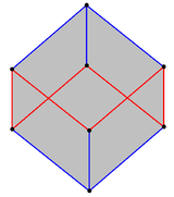
Dissections

Coxeter states that every zonogon (a 2m-gon whose opposite sides are parallel and of equal length) can be dissected into ${tbinom {n}{2}}$ or m(m-1)/2 parallelograms.
These tilings are contained as subsets of vertices, edges and faces in orthogonal projections m-cubes.^[5]
In particular this is true for regular polygons with evenly many sides, in which case the parallelograms are all rhombi.
The list OEIS: A006245 gives the number of solutions for smaller polygons.

Example dissections for select even-sided regular polygons
2m	6	8	10	12	14	16	18	20	24	30	40	50
Image
Rhombs	3	6	10	15	21	28	36	45	66	105	190	300

Area

The area A of a convex regular n-sided polygon having side s, circumradius R, apothem a, and perimeter p is given by^[6]^[7]

{displaystyle A={tfrac {1}{2}}nsa={tfrac {1}{2}}pa={tfrac {1}{4}}ns^{2}cot left({tfrac {pi }{n}}right)=na^{2}tan left({tfrac {pi }{n}}right)={tfrac {1}{2}}nR^{2}sin left({tfrac {2pi }{n}}right)}

For regular polygons with side s = 1, circumradius R = 1, or apothem a = 1, this produces the following table:^[8] (Note that since ${displaystyle cot xrightarrow 1/x}$ as $x rightarrow 0$ ^[9], the area when $s=1$ is tending to ${displaystyle n^{2}/4pi }$ as $n$ grows large.)

Number of sides	Area when side s = 1		Area when circumradius R = 1			Area when apothem a = 1
Number of sides	Exact	Approximation	Exact	Approximation	As an (approximate) fraction of circumcircle area	Exact	Approximation	As an (approximate) multiple of incircle area
n	${displaystyle {tfrac {n}{4}}cot left({tfrac {pi }{n}}right)}$		${displaystyle {tfrac {n}{2}}sin left({tfrac {2pi }{n}}right)}$		${displaystyle {tfrac {n}{2pi }}sin left({tfrac {2pi }{n}}right)}$	${displaystyle ntan left({tfrac {pi }{n}}right)}$		${displaystyle {tfrac {n}{pi }}tan left({tfrac {pi }{n}}right)}$
3	${displaystyle {tfrac {sqrt {3}}{4}}}$	0.433012702	${displaystyle {tfrac {3{sqrt {3}}}{4}}}$	1.299038105	0.4134966714	${displaystyle 3{sqrt {3}}}$	5.196152424	1.653986686
4	1	1.000000000	2	2.000000000	0.6366197722	4	4.000000000	1.273239544
5	${displaystyle {tfrac {1}{4}}{sqrt {25+10{sqrt {5}}}}}$	1.720477401	${displaystyle {tfrac {5}{4}}{sqrt {{tfrac {1}{2}}left(5+{sqrt {5}}right)}}}$	2.377641291	0.7568267288	${displaystyle 5{sqrt {5-2{sqrt {5}}}}}$	3.632712640	1.156328347
6	${displaystyle {tfrac {3{sqrt {3}}}{2}}}$	2.598076211	${displaystyle {tfrac {3{sqrt {3}}}{2}}}$	2.598076211	0.8269933428	${displaystyle 2{sqrt {3}}}$	3.464101616	1.102657791
7		3.633912444		2.736410189	0.8710264157		3.371022333	1.073029735
8	${displaystyle 2+2{sqrt {2}}}$	4.828427125	${displaystyle 2{sqrt {2}}}$	2.828427125	0.9003163160	${displaystyle 8left({sqrt {2}}-1right)}$	3.313708500	1.054786175
9		6.181824194		2.892544244	0.9207254290		3.275732109	1.042697914
10	${displaystyle {tfrac {5}{2}}{sqrt {5+2{sqrt {5}}}}}$	7.694208843	${displaystyle {tfrac {5}{2}}{sqrt {{tfrac {1}{2}}left(5-{sqrt {5}}right)}}}$	2.938926262	0.9354892840	${displaystyle 2{sqrt {25-10{sqrt {5}}}}}$	3.249196963	1.034251515
11		9.365639907		2.973524496	0.9465022440		3.229891423	1.028106371
12	${displaystyle 6+3{sqrt {3}}}$	11.19615242	3	3.000000000	0.9549296586	${displaystyle 12left(2-{sqrt {3}}right)}$	3.215390309	1.023490523
13		13.18576833		3.020700617	0.9615188694		3.204212220	1.019932427
14		15.33450194		3.037186175	0.9667663859		3.195408642	1.017130161
15	^[10]	17.64236291	^[11]	3.050524822	0.9710122088	^[12]	3.188348426	1.014882824
16	^[13]	20.10935797	${displaystyle 4{sqrt {2-{sqrt {2}}}}}$	3.061467460	0.9744953584	^[14]	3.182597878	1.013052368
17		22.73549190		3.070554163	0.9773877456		3.177850752	1.011541311
18		25.52076819		3.078181290	0.9798155361		3.173885653	1.010279181
19		28.46518943		3.084644958	0.9818729854		3.170539238	1.009213984
20	^[15]	31.56875757	^[16]	3.090169944	0.9836316430	^[17]	3.167688806	1.008306663
100		795.5128988		3.139525977	0.9993421565		3.142626605	1.000329117
1000		79577.20975		3.141571983	0.9999934200		3.141602989	1.000003290
10,000		7957746.893		3.141592448	0.9999999345		3.141592757	1.000000033
1,000,000		79577471545		3.141592654	1.000000000		3.141592654	1.000000000

Of all n-gons with a given perimeter, the one with the largest area is regular.^[18]

Constructible polygon

Some regular polygons are easy to construct with compass and straightedge; other regular polygons are not constructible at all.
The ancient Greek mathematicians knew how to construct a regular polygon with 3, 4, or 5 sides,^[19]^{:p. xi} and they knew how to construct a regular polygon with double the number of sides of a given regular polygon.^[19]^{:pp. 49–50} This led to the question being posed: is it possible to construct all regular n-gons with compass and straightedge? If not, which n-gons are constructible and which are not?

Carl Friedrich Gauss proved the constructibility of the regular 17-gon in 1796. Five years later, he developed the theory of Gaussian periods in his Disquisitiones Arithmeticae. This theory allowed him to formulate a sufficient condition for the constructibility of regular polygons:

A regular n-gon can be constructed with compass and straightedge if n is the product of a power of 2 and any number of distinct Fermat primes (including none).

(A Fermat prime is a prime number of the form $2^{{(2^{n})}}+1.$ ) Gauss stated without proof that this condition was also necessary, but never published his proof. A full proof of necessity was given by Pierre Wantzel in 1837. The result is known as the Gauss–Wantzel theorem.

Equivalently, a regular n-gon is constructible if and only if the cosine of its common angle is a constructible number—that is, can be written in terms of the four basic arithmetic operations and the extraction of square roots.

Regular skew polygons

The cube contains a skew regular hexagon, seen as 6 red edges zig-zagging between two planes perpendicular to the cube's diagonal axis.	The zig-zagging side edges of a n-antiprism represent a regular skew 2n-gon, as shown in this 17-gonal antiprism.

A regular skew polygon in 3-space can be seen as nonplanar paths zig-zagging between two parallel planes, defined as the side-edges of a uniform antiprism. All edges and internal angles are equal.

The Platonic solids (the tetrahedron, cube, octahedron, dodecahedron, and icosahedron) have Petrie polygons, seen in red here, with sides 4, 6, 6, 10, and 10 respectively.

More generally regular skew polygons can be defined in n-space. Examples include the Petrie polygons, polygonal paths of edges that divide a regular polytope into two halves, and seen as a regular polygon in orthogonal projection.

In the infinite limit regular skew polygons become skew apeirogons.

Regular star polygons

2 < 2q < p, gcd(p, q) = 1

{5/2}	{7/2}	{7/3}...

Schläfli symbol

{p/q}

Vertices and Edges

p

Density

q

Coxeter diagram

Symmetry group

Dihedral (D_p)

Dual polygon

Self-dual

Internal angle
(degrees)

{displaystyle {frac {180(p-2q)}{p}}}

^[20]

A non-convex regular polygon is a regular star polygon. The most common example is the pentagram, which has the same vertices as a pentagon, but connects alternating vertices.

For an n-sided star polygon, the Schläfli symbol is modified to indicate the density or "starriness" m of the polygon, as {n/m}. If m is 2, for example, then every second point is joined. If m is 3, then every third point is joined. The boundary of the polygon winds around the center m times.

The (non-degenerate) regular stars of up to 12 sides are:

Pentagram – {5/2}

Heptagram – {7/2} and {7/3}

Octagram – {8/3}

Enneagram – {9/2} and {9/4}

Decagram – {10/3}

Hendecagram – {11/2}, {11/3}, {11/4} and {11/5}

Dodecagram – {12/5}

m and n must be coprime, or the figure will degenerate.

The degenerate regular stars of up to 12 sides are:

Tetragon – {4/2}

Hexagons – {6/2}, {6/3}

Octagons – {8/2}, {8/4}

Enneagon – {9/3}

Decagons – {10/2}, {10/4}, and {10/5}

Dodecagons – {12/2}, {12/3}, {12/4}, and {12/6}

Two interpretations of {6/2}
Grünbaum {6/2} or 2{3}^[21]	Coxeter 2{3} or {6}[2{3}]{6}

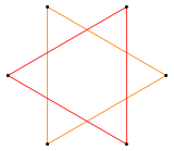Doubly-wound hexagon	Hexagram as a compound of two triangles

Depending on the precise derivation of the Schläfli symbol, opinions differ as to the nature of the degenerate figure. For example, {6/2} may be treated in either of two ways:

For much of the 20th century (see for example Coxeter (1948)), we have commonly taken the /2 to indicate joining each vertex of a convex {6} to its near neighbors two steps away, to obtain the regular compound of two triangles, or hexagram.
Coxeter clarifies this regular compound with a notation {kp}[k{p}]{kp} for the compound {p/k}, so the hexagram is represented as {6}[2{3}]{6}.^[22] More compactly Coxeter also writes 2{n/2}, like 2{3} for a hexagram as compound as alternations of regular even-sided polygons, with italics on the leading factor to differentiate it from the coinciding interpretation.^[23]

Many modern geometers, such as Grünbaum (2003),^[21] regard this as incorrect. They take the /2 to indicate moving two places around the {6} at each step, obtaining a "double-wound" triangle that has two vertices superimposed at each corner point and two edges along each line segment. Not only does this fit in better with modern theories of abstract polytopes, but it also more closely copies the way in which Poinsot (1809) created his star polygons – by taking a single length of wire and bending it at successive points through the same angle until the figure closed.

Duality of regular polygons

All regular polygons are self-dual to congruency, and for odd n they are self-dual to identity.

In addition, the regular star figures (compounds), being composed of regular polygons, are also self-dual.

Regular polygons as faces of polyhedra

A uniform polyhedron has regular polygons as faces, such that for every two vertices there is an isometry mapping one into the other (just as there is for a regular polygon).

A quasiregular polyhedron is a uniform polyhedron which has just two kinds of face alternating around each vertex.

A regular polyhedron is a uniform polyhedron which has just one kind of face.

The remaining (non-uniform) convex polyhedra with regular faces are known as the Johnson solids.

A polyhedron having regular triangles as faces is called a deltahedron.

Notes

^ Park, Poo-Sung. "Regular polytope distances", Forum Geometricorum 16, 2016, 227-232. http://forumgeom.fau.edu/FG2016volume16/FG201627.pdf

^ ^a^b^c^d Johnson, Roger A., Advanced Euclidean Geometry, Dover Publ., 2007 (orig. 1929).

^ Pickover, Clifford A, The Math Book, Sterling, 2009: p. 150

^ Chen, Zhibo, and Liang, Tian. "The converse of Viviani's theorem", The College Mathematics Journal 37(5), 2006, pp. 390–391.

^ Coxeter, Mathematical recreations and Essays, Thirteenth edition, p.141

^ "Math Open Reference". Retrieved 4 Feb 2014..mw-parser-output cite.citation{font-style:inherit}.mw-parser-output q{quotes:"""""""'""'"}.mw-parser-output code.cs1-code{color:inherit;background:inherit;border:inherit;padding:inherit}.mw-parser-output .cs1-lock-free a{background:url("//upload.wikimedia.org/wikipedia/commons/thumb/6/65/Lock-green.svg/9px-Lock-green.svg.png")no-repeat;background-position:right .1em center}.mw-parser-output .cs1-lock-limited a,.mw-parser-output .cs1-lock-registration a{background:url("//upload.wikimedia.org/wikipedia/commons/thumb/d/d6/Lock-gray-alt-2.svg/9px-Lock-gray-alt-2.svg.png")no-repeat;background-position:right .1em center}.mw-parser-output .cs1-lock-subscription a{background:url("//upload.wikimedia.org/wikipedia/commons/thumb/a/aa/Lock-red-alt-2.svg/9px-Lock-red-alt-2.svg.png")no-repeat;background-position:right .1em center}.mw-parser-output .cs1-subscription,.mw-parser-output .cs1-registration{color:#555}.mw-parser-output .cs1-subscription span,.mw-parser-output .cs1-registration span{border-bottom:1px dotted;cursor:help}.mw-parser-output .cs1-hidden-error{display:none;font-size:100%}.mw-parser-output .cs1-visible-error{font-size:100%}.mw-parser-output .cs1-subscription,.mw-parser-output .cs1-registration,.mw-parser-output .cs1-format{font-size:95%}.mw-parser-output .cs1-kern-left,.mw-parser-output .cs1-kern-wl-left{padding-left:0.2em}.mw-parser-output .cs1-kern-right,.mw-parser-output .cs1-kern-wl-right{padding-right:0.2em}

^ "Mathwords".

^ Results for R = 1 and a = 1 obtained with Maple, using function definition:

f := proc (n)

options operator, arrow;

[

 [convert(1/4*n*cot(Pi/n), radical), convert(1/4*n*cot(Pi/n), float)],

 [convert(1/2*n*sin(2*Pi/n), radical), convert(1/2*n*sin(2*Pi/n), float), convert(1/2*n*sin(2*Pi/n)/Pi, float)],

 [convert(n*tan(Pi/n), radical), convert(n*tan(Pi/n), float), convert(n*tan(Pi/n)/Pi, float)]

]

end proc

The expressions for n=16 are obtained by twice applying the tangent half-angle formula to tan(π/4)

^ Trigonometric functions

^ ${displaystyle {tfrac {15}{8}}left({sqrt {15}}+{sqrt {3}}+{sqrt {2left(5+{sqrt {5}}right)}}right)}$

^ ${displaystyle {tfrac {15}{16}}left({sqrt {15}}+{sqrt {3}}-{sqrt {10-2{sqrt {5}}}}right)}$

^ ${displaystyle {tfrac {15}{2}}left(3{sqrt {3}}-{sqrt {15}}-{sqrt {2left(25-11{sqrt {5}}right)}}right)}$

^ ${displaystyle 4left(1+{sqrt {2}}+{sqrt {2left(2+{sqrt {2}}right)}}right)}$

^ ${displaystyle 16left(1+{sqrt {2}}right)left({sqrt {2left(2-{sqrt {2}}right)}}-1right)}$

^ ${displaystyle 5left(1+{sqrt {5}}+{sqrt {5+2{sqrt {5}}}}right)}$

^ ${displaystyle {tfrac {5}{2}}left({sqrt {5}}-1right)}$

^ ${displaystyle 20left(1+{sqrt {5}}-{sqrt {5+2{sqrt {5}}}}right)}$

^ Chakerian, G.D. "A Distorted View of Geometry." Ch. 7 in Mathematical Plums (R. Honsberger, editor). Washington, DC: Mathematical Association of America, 1979: 147.

^ ^a^b Bold, Benjamin. Famous Problems of Geometry and How to Solve Them, Dover Publications, 1982 (orig. 1969).

^ Kappraff, Jay (2002). Beyond measure: a guided tour through nature, myth, and number. World Scientific. p. 258. ISBN 978-981-02-4702-7.

^ ^a^b Are Your Polyhedra he Same as My Polyhedra? Branko Grünbaum (2003), Fig. 3

^ Regular polytopes, p.95

^ Coxeter, The Densities of the Regular Polytopes II, 1932, p.53

References

Coxeter, H.S.M. (1948). "Regular Polytopes". Methuen and Co.

Grünbaum, B.; Are your polyhedra the same as my polyhedra?, Discrete and comput. geom: the Goodman-Pollack festschrift, Ed. Aronov et al., Springer (2003), pp. 461–488.

Poinsot, L.; Memoire sur les polygones et polyèdres. J. de l'École Polytechnique 9 (1810), pp. 16–48.

External links

Weisstein, Eric W. "Regular polygon". MathWorld.

Regular Polygon description With interactive animation

Incircle of a Regular Polygon With interactive animation

Area of a Regular Polygon Three different formulae, with interactive animation

Renaissance artists' constructions of regular polygons at Convergence

v t e Fundamental convex regular and uniform polytopes in dimensions 2–10
Family	A_n	B_n	I₂(p) / D_n	E₆ / E₇ / E₈ / F₄ / G₂	H_n
Regular polygon	Triangle	Square	p-gon	Hexagon	Pentagon
Uniform polyhedron	Tetrahedron	Octahedron • Cube	Demicube		Dodecahedron • Icosahedron
Uniform 4-polytope	5-cell	16-cell • Tesseract	Demitesseract	24-cell	120-cell • 600-cell
Uniform 5-polytope	5-simplex	5-orthoplex • 5-cube	5-demicube
Uniform 6-polytope	6-simplex	6-orthoplex • 6-cube	6-demicube	1₂₂ • 2₂₁
Uniform 7-polytope	7-simplex	7-orthoplex • 7-cube	7-demicube	1₃₂ • 2₃₁ • 3₂₁
Uniform 8-polytope	8-simplex	8-orthoplex • 8-cube	8-demicube	1₄₂ • 2₄₁ • 4₂₁
Uniform 9-polytope	9-simplex	9-orthoplex • 9-cube	9-demicube
Uniform 10-polytope	10-simplex	10-orthoplex • 10-cube	10-demicube
Uniform n-polytope	n-simplex	n-orthoplex • n-cube	n-demicube	1_k2 • 2_k1 • k₂₁	n-pentagonal polytope
Topics: Polytope families • Regular polytope • List of regular polytopes and compounds

[1] Park, Poo-Sung. "Regular polytope distances", Forum Geometricorum 16, 2016, 227-232. http://forumgeom.fau.edu/FG2016volume16/FG201627.pdf

[Johnson-2] Johnson, Roger A., Advanced Euclidean Geometry, Dover Publ., 2007 (orig. 1929).

[3] Pickover, Clifford A, The Math Book, Sterling, 2009: p. 150

[4] Chen, Zhibo, and Liang, Tian. "The converse of Viviani's theorem", The College Mathematics Journal 37(5), 2006, pp. 390–391.

[5] Coxeter, Mathematical recreations and Essays, Thirteenth edition, p.141

[6] "Math Open Reference". Retrieved 4 Feb 2014..mw-parser-output cite.citation{font-style:inherit}.mw-parser-output q{quotes:"""""""'""'"}.mw-parser-output code.cs1-code{color:inherit;background:inherit;border:inherit;padding:inherit}.mw-parser-output .cs1-lock-free a{background:url("//upload.wikimedia.org/wikipedia/commons/thumb/6/65/Lock-green.svg/9px-Lock-green.svg.png")no-repeat;background-position:right .1em center}.mw-parser-output .cs1-lock-limited a,.mw-parser-output .cs1-lock-registration a{background:url("//upload.wikimedia.org/wikipedia/commons/thumb/d/d6/Lock-gray-alt-2.svg/9px-Lock-gray-alt-2.svg.png")no-repeat;background-position:right .1em center}.mw-parser-output .cs1-lock-subscription a{background:url("//upload.wikimedia.org/wikipedia/commons/thumb/a/aa/Lock-red-alt-2.svg/9px-Lock-red-alt-2.svg.png")no-repeat;background-position:right .1em center}.mw-parser-output .cs1-subscription,.mw-parser-output .cs1-registration{color:#555}.mw-parser-output .cs1-subscription span,.mw-parser-output .cs1-registration span{border-bottom:1px dotted;cursor:help}.mw-parser-output .cs1-hidden-error{display:none;font-size:100%}.mw-parser-output .cs1-visible-error{font-size:100%}.mw-parser-output .cs1-subscription,.mw-parser-output .cs1-registration,.mw-parser-output .cs1-format{font-size:95%}.mw-parser-output .cs1-kern-left,.mw-parser-output .cs1-kern-wl-left{padding-left:0.2em}.mw-parser-output .cs1-kern-right,.mw-parser-output .cs1-kern-wl-right{padding-right:0.2em}

[7] "Mathwords".

[8] Results for R = 1 and a = 1 obtained with Maple, using function definition:

f := proc (n)
options operator, arrow;
[
[convert(1/4*n*cot(Pi/n), radical), convert(1/4*n*cot(Pi/n), float)],
[convert(1/2*n*sin(2*Pi/n), radical), convert(1/2*n*sin(2*Pi/n), float), convert(1/2*n*sin(2*Pi/n)/Pi, float)],
[convert(n*tan(Pi/n), radical), convert(n*tan(Pi/n), float), convert(n*tan(Pi/n)/Pi, float)]
]
end proc

The expressions for n=16 are obtained by twice applying the tangent half-angle formula to tan(π/4)

[9] Trigonometric functions

[10] ${displaystyle {tfrac {15}{8}}left({sqrt {15}}+{sqrt {3}}+{sqrt {2left(5+{sqrt {5}}right)}}right)}$

[11] ${displaystyle {tfrac {15}{16}}left({sqrt {15}}+{sqrt {3}}-{sqrt {10-2{sqrt {5}}}}right)}$

[12] ${displaystyle {tfrac {15}{2}}left(3{sqrt {3}}-{sqrt {15}}-{sqrt {2left(25-11{sqrt {5}}right)}}right)}$

[13] ${displaystyle 4left(1+{sqrt {2}}+{sqrt {2left(2+{sqrt {2}}right)}}right)}$

[14] ${displaystyle 16left(1+{sqrt {2}}right)left({sqrt {2left(2-{sqrt {2}}right)}}-1right)}$

[15] ${displaystyle 5left(1+{sqrt {5}}+{sqrt {5+2{sqrt {5}}}}right)}$

[16] ${displaystyle {tfrac {5}{2}}left({sqrt {5}}-1right)}$

[17] ${displaystyle 20left(1+{sqrt {5}}-{sqrt {5+2{sqrt {5}}}}right)}$

[18] Chakerian, G.D. "A Distorted View of Geometry." Ch. 7 in Mathematical Plums (R. Honsberger, editor). Washington, DC: Mathematical Association of America, 1979: 147.

[Bold-19] Bold, Benjamin. Famous Problems of Geometry and How to Solve Them, Dover Publications, 1982 (orig. 1969).

[20] Kappraff, Jay (2002). Beyond measure: a guided tour through nature, myth, and number. World Scientific. p. 258. ISBN 978-981-02-4702-7.

[Branko-21] Are Your Polyhedra he Same as My Polyhedra? Branko Grünbaum (2003), Fig. 3

[22] Regular polytopes, p.95

[23] Coxeter, The Densities of the Regular Polytopes II, 1932, p.53

v t e Polygons (List)
1–10 sides	Monogon Digon Triangle Equilateral Isosceles Right Acute/Obtuse Quadrilateral Square Rectangle Rhombus Parallelogram Trapezoid Isosceles trapezoid Kite Pentagon Hexagon Heptagon Octagon Nonagon (Enneagon) Decagon
11–20 sides	Hendecagon Dodecagon Tridecagon Tetradecagon Pentadecagon Hexadecagon Heptadecagon Octadecagon Enneadecagon Icosagon
21–100 sides (selected)	Icosidigon (22) Icositetragon (24) Icosihexagon (26) Icosioctagon (28) Triacontagon (30) Triacontadigon (32) Triacontatetragon (34) Tetracontagon (40) Tetracontadigon (42) Tetracontaoctagon (48) Pentacontagon (50) Hexacontagon (60) Hexacontatetragon (64) Heptacontagon (70) Octacontagon (80) Enneacontagon (90) Enneacontahexagon (96) Hectogon (100)
>100 sides	120-gon 257-gon 360-gon Chiliagon (1000) Myriagon (10000) 65537-gon Megagon (1000000) Apeirogon (∞)
Star polygons (5–12 sides)	Pentagram Hexagram Heptagram Octagram Enneagram Decagram Hendecagram Dodecagram
Others	Pseudogon Skew polygon Skew apeirogon
Classes	Concave Convex Cyclic Equiangular Equilateral Isogonal Isotoxal Regular Simple Tangential

搜尋此網誌